Transcription
QGIS Interface forSWAT (QSWAT)Version 1.9August 2019Prepared by: Yihun Dile, R. Srinivasan and Chris GeorgeThis guide describes QSWAT, which uses the 2012 version of the SWAT model.This version describes QSWAT version 1.8.2, which needs SWAT Editor version 2012.10.21.1
QSWAT (QGIS SWAT)Step by Step Setup for the Robit Watershed, Lake Tana basinEthiopiaContents1.Environment and Tools Required . 42.Installation. 43.Structure and Location of Source Data . 64.Structure and Location of Output Data . 75.Setup for Robit Watershed, Lake Tana Basin . 85.1.Watershed Delineation . 105.2.Create HRUs . 205.3.SWAT Setup and Run . 325.4.Output Visualisation with QSWAT. 375.4.1. Preparing to visualise . 385.4.2. Running visualise . 385.4.3. Visualisation period. 395.4.4. Static visualisation . 395.4.5 Printing. 425.4.6 Animation. 495.4.7. Plotting . 575.5.67SWAT Output Visualization with SWAT Error Checker . 62Appendix I . 676.1Adding tables into SWAT reference database . 676.2Preparing daily climatic data for QSWAT . 716.3Preparing landuse and soil look-up tables . 73Appendix II – preparing global DEM data for QSWAT . 747.1Introduction . 747.2Obtaining SRTM DEM data . 747.2.1.90m data . 742
7.2.2.30m data . 747.3.Clipping the grids . 757.4.Merging the grids . 767.5.Reprojecting the grid . 777.6.Masking a DEM . 817.7.Large DEMs . 848Appendix III: Using a Predefined Watershed and Stream Network . 879Appendix IV: Installing and Using MPI . 90Installing MS-MPI. 909.2Configuring QSWAT to use MPI . 919.3Blocking network access . 91109.1Appendix V: Converting ArcSWAT Projects to QSWAT . 93 Purpose . 93 Instructions . 9410.2.1Prerequisites . 9410.2.2Conversion . 94 Other data . 983
1. Environment and Tools Required Microsoft Windows (any version, as far as we are aware)Microsoft Access, as the interface uses an Access databaseText editor (e.g. WordPad, NotePad, NotePad ) that enables you to read and edit ASCIItext files.A tool like WinZip that can uncompress.zip files (not needed with recent versions ofWindows)System requirements for SWAT Editor Version 2012.10.19 Microsoft Windows XP to 10 Microsoft .Net Framework 3.5 Adobe Acrobat Reader Version 7 or higher. Acrobat Reader may be downloaded for freefrom: ml2. Installation Install QGIS by running QGIS-OSGeo4W-2.6.1-1-Setup-x86.exe. It can be downloadedfrom up-x86.exe. Use the defaultfolder C:\Program Files\QGIS Brighton as the installation folder, or C:\Program Files(x86)\QGIS Brighton on a 64-bit machine. Currently you must use the 32-bit version on64-bit machines. We recommend version 2.6 rather than a later version. From now on wewill use Program Files as a folder name, even though it will be Program Files (x86) on a64-bit machine.Install SWATEditor 2012 version in its standard place C:\SWAT\SWATEditor. For veSwateditor Install 2012.19 5.21.zip (or a later version if available or/) and double-click on the "setup.exe"program to install the SWAT Editor. This will launch the SWAT Editor install program.Use the default folder C:\SWAT\SWATEditor as the installation folder.The SWATEditor folder will consist of Databases folder, SwatCheck folder,SWATEditorHelp, and other SWAT executables. The database folder consists of SWAT2012databases which require updating based on user available information (e.g. user soil, weathergenerator). Refer to Appendix I (page 67) on how to update a database. Refer to theSWATEditor Documentation.pdf document in SWATEditorHelp for important informationon how to get started with the SWAT Editor.4
WARNING. If you use this version 1.7 or later of QSWAT on a project developed with anolder version of QSWAT, then the reference database stored in the project directory will needupdating. There are two ways to do this: After installing QSWAT 1.7 you can copy the new reference mdb to your project folder,overwriting the file of the same name there. If you have made any changes to your project's reference database, such as your ownusersoil table, it may be easier to update your database. You can do this when youstart the SWAT Editor, before you start writing tables. Having started the editor andconnected to databases, Select Write Input Tables, then Database Update. Select thebsn table, make sure Update SWAT Range Tables is selected, and click UpdateDatabase. Do the same thing for the rte table.Make sure you have the system requirements listed above for the SWAT Editor to workproperly. Failure to have the above system configuration may result in failure to install theSWAT Editor or errors in the SWAT Editor interface.Users can join the user group for help at https://groups.google.com/forum/#!forum/qswat5
Figure 1: SWAT Editor installation folder (after installing QSWAT) Install QSWAT by running QSWATinstall1.7.exe or a later version. This adds some filesto the SWATEditor: a project database and a reference database in Databases, and alsostores the TauDEM executables in a new folder C:\SWAT\SWATEditor\TauDEM5Bin. TheQGIS plugin QSWAT is put into the user's home folder in .qgis2\python\plugins\QSWAT,which we will refer to as the QSWAT folder. The latest version of QSWAT can bedownloaded from the SWAT website http://swat.tamu.edu/.3. Structure and Location of Source Data6
Before starting QGIS, users should prepare their tabular and spatial data according to SWAT requirements. Users can refer to Appendix I (page 67) on preparing tabular data (e.g. preparingsoil and climatic data). All the spatial data (DEM, land use and soil) should be projected into thesame projected coordinate system. Users can refer to Appendix II (page 74) for preparing globaldata for QSWAT. Users can also refer to the Arcswat Interface for SWAT2012 User’s Guide(pages 11-36) for detailed guidance. The example files used in this manual are available in theQSWAT folder in a folder ExampleDataset. This folder contains: A DEM in folder DEM A stream reaches file to burn in to the DEM, in folder RobitStreams An outlet file in folder MainOutlet Landuse and soil maps in directories Landuse and Soil Climate data in folder ClimateRobit Some Excel and csv files for making database tables, and An observed data file observedFlow.csv in folder Observed.It is a good idea while following this guide to add the ExampleDataset folder to your Favoritesor Quick Access list, as we will be regularly accessing files within it.4. Structure and Location of Output DataWe will be establishing a project called Demo, say, in a folder C:\ QSWAT Projects\Robit\Demo.This will create:1) In the folder C:\QSWAT Projects\Robit the project file Demo.qgs and a folder Demo.If we later want to reopen the project Demo.qgs will be the file we look for. Thefolder Demo is the project folder.2) A folder C:\QSWAT Projects\Robit\Demo\Scenarios\Default\TxtInOut that willcontain all the SWAT input and output files.3) A folder C:\QSWAT Projects\Robit\Demo\Scenarios\Default\TablesIn that may beused by the SWAT Editor.4) A folder C:\QSWAT Projects\Robit\Demo\Scenarios\Default\TablesOut that may beused by the SWAT Editor and is used to hold results files from visualisation.5) A folder C:\QSWAT Projects\Robit\Demo\Source that will contain copies of our inputmaps and a number of intermediate maps generated during watershed delineation.6) If we choose to save a SWAT run as Sim1, say, then a folderC:\QSWAT Projects\Robit\Demo\Scenarios\Sim1 will be created (a copy ofC:\QSWAT Projects\Robit\Demo\Scenarios\Default, including its sub-folders).7) A folder C:\QSWAT Projects\Robit\Demo\Watershed with several sub-folders7
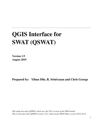
5. Setup for Robit Watershed, Lake Tana Basin1. Start QGIS and select Plugins menu Manage and Install Plugins and findQSWAT. Click its checkbox to install, which takes a few seconds. The SWAT iconwill appear in the toolbar. If it fails to appear check you are running a 32 bit versionof QGIS.SWATFigure 2; QGIS with the SWAT icon2.Start QSWAT by clicking the SWAT icon.3.The main QSWAT interface will be displayed. Click the box New Project.4.A browser will be displayed requesting a name for the new project. Type Demo in thetext box labelled File name (under the C:\QSWAT Projects\Robit folder). See Figure 3.8
Figure 3: Creating a QSWAT projectAt this stage all your maps should be prepared in an equal area projection (probably, but notnecessarily, UTM1). All the maps should be in the same projection coordinate system.The interface now presents a step-by-step configuration to be followed in order to prepare theSWAT simulation, starting with Step 1 (Figure 4).1UTM is not an equal area projection, but is close to being so, and sufficiently close for SWAT to use on mostwatersheds.9
Figure 4: Step 1 interface5.At this stage the project database is created as Demo.mdb in the project folder, and a copyof the SWAT reference database QSWATRef2012.mdb is also created there. For this example youneed to update the reference database with details of the soil data we are using and also possibleweather generation stations. Refer to Appendix I (page 67) on how to do this.5.1.Watershed Delineation6.To start automatic watershed delineation click the Delineate Watershed button. Whenthe prompt box is opened browse to the data source in the dialogue box next to Select DEM.7.Browse to the ExampleDataset\DEM\srtm 30m folder and open the file hdr.adf. Thisdigital elevation map (DEM) is an ESRI grid and consists of a number of files. The file calledhdr.adf is the one to choose for such a grid. DEMs are raster files (also called grids) and comein a large variety of formats. A common format is GeoTiff, when you would be looking for afile with siffix .tif.10
Figure 5: Selecting the DEM8.The name of the elevation map grid will be displayed in the DEM text box below theWatershed dialogue box. The selected DEM will be copied to the projects Source folder and, ifnecessary, converted to GeoTiff format (.tif). If your DEM's units are not metres you can selectthe DEM properties tab and change them. This tab also shows the DEM cell size, cell area,projection system and extent in degrees.9.Users can burn in an existing stream network using the option Burn in existing streamnetwork; use a file with the extension *.shp (Figure 6). Check the Burn in existing streamnetwork option and select the file ExampleDataset\RobitStreams\robReach.shp.The delineation form allows you to opt for a predefined watershed and stream network byselecting the Use existing watershed tab. If you are interested in using a predefined watershedand stream network please refer to Appendix III (Using a Predefined Watershed and StreamNetwork, page 87).We will not use MPI, which enables multiprocessing during watershed delineation (see Appendix11
IV, page 90) and so the Number of processes spinbox should be set to 0.Figure 6: Creating stream networks10.The threshold size for creating subbasins should be set next. It can be set by area, invarious units such as sq km or hectares, or by number of cells. If necessary, change the threshold12
method to use hectares, change the number of hectares to 90, and press Create Streams: thenumber of cells will be adjusted to the corresponding value (1000). The threshold is the numberof cells (or area) required to form a stream: a cell will be made part of a stream if it has at leastthe threshold number of cells draining into it. Stream reaches are sections of the stream networkbetween significant points, where significant points are stream sources, stream junctions, andinlet, outlet, point source, and reservoir points that we may add later. A subbasin is an areadraining into a stream reach. This step creates streams (Figure 7). It also loads the stream burn-inshapefile if selected.Figure 7: Stream networks displayed11.An inlets/outlets file containing just a main outlet is provided for this example. Check theUse an inlets/outlets shapefile option, and browse to MainOutlet/MainOutlet.shp12.Users can add outlets, reservoirs, inlets, and point sources by selecting the DrawInlets/Outlets option. This first asks if you wish to add to the existing inlets/outlets file, or createa new one. Having made this choice, select the type of point to add, and click on the map to13
place it at the appropriate place. Points need to be placed on the stream network, and you mayneed to zoom in to place them precisely. Only points within the snap threshold of a stream reachwill be counted as points. Click OK to confirm and exit, and Cancel to remove points and exit.If you choose to draw, a new file, drawoutlets.shp is created in the Watershed\Shapes folder,which may be used again. See Appendix III (page 87) for details of the fields needed in aninlets/outlets file. We do not add any additional outlets, reservoirs, inlets, or point sources in thisexample.Figure 8: Step where Inlets/Outlets are added.13.If you have several points in your inlets/outlets file you can choose to use just a selectionof them. To do this choose the Select Inlets/Outlets option. Hold Ctrl and select the points bydragging the mouse to make a small rectangle around them. Selected points will turn yellow, anda count will be shown at the bottom left of the main window (Figure 9). You only need to use thisoption if you want to only use a subset of outlets. The default is to use all the points in theoutlets file or those drawn.14
Figure 9: .Inlets/outlets selected14.Clicking Review snapped shows the snapped inlets/outlets, i.e. those within the definedthreshold distance. Clicking Create Watershed will create the watershed after a few minutes(Figure 10).15
Figure 10: Delineated watersheds15.In QSWAT users can select and merge subbasins. This is especially important in avoidingsmall subbasins. To merge subbasins, select the option Select subbasins under Merge subbasins.Hold the Ctrl key and click in subbasins you want to select. Selected subbasins will turn yellow,and a count is shown at the bottom left of the dialogue window (Figure 11).16
Figure 11: Step of merging subbasins16.For the sake of this exercise, we will not merge the selected subbasin. Release the Ctrlkey and click on the map outside the watershed and the selected subbasin will be unselected.Checking the option of Select small subbasins provides the option to merge subbasins below acertain threshold (i.e. either the area in hectares or a percentage of the mean subbasin area)(Figure 12). For this exercise click the radio button percentage of mean area, and put 25 in thebox next to it. Click Select. It will show you subbasins that have an area less than 25% of themean area. When finished click Save to save your selection, or Cancel to abandon your selection.You click Merge to perform the merge. Note: You cannot merge a subbasin that has an outlet,inlet, reservoir, or point source. So in this example, the only small subbasin is that nearest thewatershed outlet, which cannot be merged, and QSWAT will report this.17
Figure 12: Subbasins that have an area less than 25% of the mean subbasin area merged to downstreamsubbasins17.Point sources can be added to all the subbasins by checking the option Add point sourceto each subbasin (Figure 13). You can also add reservoirs to selected subbasins. You then needto click Add. Unlike points added earlier, these extra point sources or reservoirs do not createsubbasin boundaries, but are added to existing subbasins, provided they do not already havepoint sources or reservoirs. Adding point sources to all subbasins is useful if you have several toadd. It is quite safe since only those you provide input data for will have any effect on the SWATsimulation.18
Figure 13: Point sources added to each subbasin18.You need to click OK. This causes the subbasins to be numbered and calculates andstores information about the subbasins and streams. This step ends watershed delineation, andenables the Create HRUs option (Figure 14).19
Figure 14: Watershed delineation is completed, and Create HRUs is enabled5.2.Create HRUs19.Having calculated the basins you needed to calculate the details of the HydrologicalResponse Units (HRUs) that are used by SWAT. These are divisions of basins into smaller unitseach of which has a particular soil/landuse (crop)/slope range combination.20.To do this we click Create HRUs, selectExampleDataset\Landuse\roblandusenew\hdr.adf as the Landuse map, and selectExampleDataset\ Soil\mowr soil90\hdr.adf as the Soil map.21.We need lookup tables to convert from the numeric values found in the landuse and soilmaps to SWAT landuse codes and soil names respectively. These lookup tables must be in theproject database. You can prepare these in advance, or use predefined ones like global landusesand global soils intended for use with the corresponding global maps, or, as we will do here,use the option to import a comma separated values (.csv) file. Lookup tables for landuse musthave the string landuse in their names; lookup tables for soils must have the string soil in theirnames, or they will not appear in the pull-down menus Landuse table and Soil tablerespectively.20
22.For landuse, select the option Use csv file in the Landuse table pull-down menu. Makethe same selection for Soil table. Make sure the Soil data option is set to usersoil. The other soildata options are for watersheds in the USA for which you are using STATSGO, STATSGO2, orSSURGO soil maps. To use STATSGO2 or SSURGO soil maps you will need to downloadSWAT US SSURGO Soils.mdb fromhttp://swat.tamu.edu/media/63316/SWAT US SSURGO Soils.zip and install it inC:\SWAT\SWATEditor\Databases. No soil lookup table is needed with STATSGO2 or SSURGO.23.We will form HRUs based on slope as well as landuse and soil. We add an intermediatepoint for slopes (e.g. 10) to divide HRUs into those with average slopes in the range 0-10% andthose with average slopes above 10%. Type 10 in the box and click Insert. The Slope bands boxshows the intermediate limit is inserted. To generate the FullHRUs shapefile, click in the checkbox.24.To read in the data from the DEM, landuse, soil and slope maps and prepare to calculateHRUs, make sure Read from maps is checked and click Read (Figure 15). There is also anoption Read from previous run. This can be used when rerunning the project, provided youhave not rerun the delineation step, and not changed the soil or landuse inputs, or the slope bands,to recover information from the project database instead of rereading the grids. Reading from thedatabase is substantially faster.21
Figure 15: Reading the land use, soil and slope maps25.In our case, we have chose to make landuse and soil lookup tables from .csv files, sowhen we click Read we are first asked to select the files. For landuse, navigate toRobit landuses.csv in ExampleDataset. This has the appropriate structure for a landuse lookuptable. Its contents are shown in Figure 16. The first line, commonly included, is ignored if its22
first field is not numeric. On each other line, the first field, delimited by a comma, is a valuefrom the landuse map. The second field is a four-letter (unless it is HAY) SWAT landuse code,as found in one of the tables crop or urban in the reference database. More than one map valuemay map to the same landuse code, but map values may not be repeated.LANDUSE ID,SWAT CODE1,WATR2,AGRL3,PAST4,FRSTFigure 16: Robit landuses.csvWhen we select the csv file, it is imported into the project database to make a new lookup table.Its name is determined as follows. First, if the file name contains landuse (as ours does) it isused as the basis. Otherwise landuse lookup is used as the basis. Second, if the basis does notexist as a table name it is used, otherwise successively 0, 1, etc is appended until an unused tablename is found and used. In our case Robit landuses will be the table name. It will be selected inthe Landuse table menu and used by default next time we run the project - we only need toimport the csv file once.26.The csv file for soils is ExampleDataset\Robit soils.csv and in the same fashion willmake a lookup table Robit soils. It maps values from our soil map to soil names found in theSNAM field of the usersoil table we made earlier in the reference database (as described inAppendix I, page 67).27.After reading the grids you will notice a number of changes to the QSWAT display(Figure 17): A Slope bands map has been created and added. This allows you to see where the areasof the two slope bands selected for this project are located. If no intermediate slope limitsare chosen this map is not created. The legends for the landuse map robelandusenew and the soil map mowr soil90 includethe landuse and soil categories from the lookup tables. A shapefile FullHRUs has been created and added. This allows users to see where in eachsubbasin the potential Hydrological Response Units (HRUs) are physically located. If, forexample, we zoom in on subbasin 2, in the Legend panel select (left button) FullHRUs,open its attribute table (right button), set the mouse to Select Feature(s) (QGIS toolbar)and click in the map canvas on the box below the number 2, then we get a view likeFigure 18. We see that this potential HRU is composed of several parts, has the landuseAGRL, the soil LVx, and the slope band 0-10. Its area of 172 ha is 50.1% of the subbasin.Close the Attribute Table Editor. Generating the FullHRUs shapefile is optional, as it can23
take some time. A count of the potential HRUs (51 in this example) is displayed whetherthis file is created or not.Figure 17: After reading grids24
Figure 18: Viewing a particular HRU28.Before you continue with HRU definition, if you look at the main QSWAT window yousee that a new item Select Report to View is available and you can choose to view just tworeports at this point, which are the Elevation and Landuse and Soil reports. The elevation reportgives information about how much land is at each elevation from the lowest to the highest, bothfor the watershed as a whole and for each subbasin (Figure 19). The landuse and soil report liststhe landuse, soil and slope-band areas for each subbasin (Figure 20).25
Figure 19: Elevation report26
Figure 20: Landuse and soil report29.At this point you have the options to split landuses, and to exempt landuses, both ofwhich will affect how HRUs are defined. Splitting landuses allows you to define more precise landuses than your landuse mapprovides. If, say, you know that in this basin 50% of the AGRL (Agricultural land generic)is used for corn, and the other 50% is used for teff, you could split AGRL into 50%CORN and 50% TEFF (Figure 21). It is possible to use the original landuse (here AGRL)as one of the sub-landuses. The percentages are integers and need to sum to 100 for eachlanduse you split. Split AGRL into 50% CORN and 50% TEFF as shown. Exempting landuses allows us to ensure that a landuse is retained in the HRU calculationeven if it falls below the thresholds we will define later. For example, we might decide toexempt the forest landuse FRST (Figure 22). Make this exemption.27
Figure 21: Splitting a landuseFigure 22: Exempting a landuse30.Once all the data has been read in and stored, the Single/Multiple HRUs choice isenabled. Dominant landuse, soil, slope and Dominant HRU options provide just one HRU foreach subbasin (i.e. option of Single HRU). Dominant landuse, soil, slope chooses the landuse28
with the biggest area in the subbasin, the soil with the biggest area in the subbasin, and the sloperange with the biggest area in the subbasin and uses them for the whole subbasin. DominantHRU selects the largest of the potential HRUs in each subbasin and makes its landuse, soil andslope range the ones chosen for the whole subbasin.The options with Filter by landuse, soil, slope; Filter by area; and Target number of HRUscreate Multiple HRUs. For the Multiple HRUs option, users can exclude HRUs that areinsignificant by considering percentage thresholds or area thresholds. The option of Filter byland use, soil and slope, will ignore any potential HRUs for which the landuse, soil or slope isless than the selected threshold. The areas of HRUs that are ignored will be redistributedproportionately amongst those that are retained. The option of Filter by area will ignore HRUsthat are below a specified threshold amount (either percent of the subbasin, or area). Finally theoption of Target number of HRUs limits the number of HRUs to a user preferred amount (i.e.between the lower limit of one HRU per subbasin and the upper one of retaining all potentialHRUs).For this exercise, use the method of Filter by land use, soil and slope and choose the Thresholdmethod of Percent of subbasin. For landuse, the value of 81 as the maximum we can chooseindicates that there is a subbasin where the maximum value for a landuse is 81%. If we chose ahigher value than 81% we would be trying to ignore all the landuse categories in that subbasin.Hence 81% is the minimum across the subbasins of the maximum landuse percentage in eachsubbasin. For this exercise, select 10% for landuse, by using the slider or by typing in the box,and click Go. The interface then computes the min-max percentage for a soil as 52%. Select 10for Soil, click Go. Similarly select 10 for slope. At this stage the user can create HRUs byclicking Create HRUs (Figure 23). The number of HRUs created (54) is reported at the top ofthe map canvas.29
Figure 23: Creating multiple HRUs by Filter by land use, soil and slope31.Create HRUs is now reported as done and the third step is enabled (Figure 24). If yourequested a Full HRUs file you will notice that an Actual HRUs file has now been added. Thiscontains the potential HRUs that were retained as actual HRUs (and
5. At this stage the project database is created as Demo.mdb in the project folder, and a copy of the SWAT reference database QSWATRef2012.mdb is also created there. For this example you need to update the reference database with details of the soil data we are using and also possible weather generation stations.