Transcription
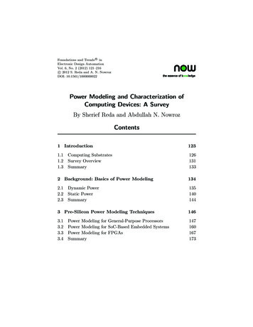
Characterization of RF andMicrowave Measurement CablesUsed with Vector NetworkAnalyzersMartin Moder and Joachim SchubertRosenberger, Fridolfing, GermanyA vector network analyzer (VNA) is as useful as the accuracy of the measurements it makes, andthis requires the instrument to be calibrated. Very often those measurements need a test setupthat includes not only the VNA and a calibration kit but also one or more measurement cablesand adapters. The calibration process employs a technique called vector error correction, inwhich error terms are characterized using known standards so that errors can be removed fromactual measurements. The process of removing these errors requires the errors and measuredquantities to be measured vectorially (thus the need for a VNA). Directly after this calibrationprocess, the best measurement accuracy can be expected. Changing anything may decreasemeasurement accuracy. Typically influences are temperature changes, bending/movement ofthe measurement cables, vibration and drift. This article concentrates on the measurementcables. It clarifies why and how cable bending and movement influence the accuracy and howmeasurement cables can be characterized to estimate their influence on the accuracy.With vector error correctionof the entire measurementsetup, the transmission andreflection behavior of themeasurement cables in magnitude andphase are mathematically removed. Subsequent movement of a measurement cablecauses small internal dimensional changes,compression of dielectric materials, changing of contact resistances and shielding. Allthese effects may result in slight changes ofthe transmission and reflection behavior sothat the vector error correction is no longerfully valid and measurement accuracy is decreased.VNA MEASUREMENT UNCERTAINTYFor different branded microwave VNAsthere are specifications for the “accuracy ofmeasurements,” “typical accuracy” or “uncertainty” in tabular and/or graphical form. Thesevalues are valid for certain combinations of aVNA type and a calibration kit type and arelimited to defined conditions such as sourcepower level and temperature change. Measurement cables are typically not included.Values of “transmission uncertainty” for ahigher end VNA in conjunction with a definedcalibration kit are shown in Figure 1. Table1 lists such uncertainties for an insertion lossrange from 0 to 20 dB taken from Figure 1.Reprinted with permission of MICROWAVE JOURNAL from the February 2022 issue. 2022 Horizon House Publications, Inc.
ApplicationNoteOne Port MeasurementsOne port measurements overcome these problemsand provide freedom in bending and movement. Measurement cables belonging to the VNA are not neces-Uncertainty (dB)50 MHz to 500 MHz500 MHz to 2 GHz2 GHz to 26.5 GHz26.5 GHz to 43.5 GHz10.10.0110S11 S22 0; Cal Power –15 dBm; Meas. Power –15 dBmIF Bandwidth 10 Hz; Average Factor 10(a)–10 –20 –30 –40 –50 –60 –70 –80 –90 –100Transmission Coefficient (dB)N5224B 400 Full Two Port Cal Using 85056D10050 MHz to 500 MHz500 MHz to 2 GHz2 GHz to 26.5 GHz26.5 GHz to 43.5 GHz101S11 S22 0; Cal Power –15 dBm; Meas. Power –15 dBmIF Bandwidth 10 Hz; Average Factor 10.110(b)0–10 –20 –30 –40 –50 –60 –70 –80 –90 –100Transmission Coefficient (dB) Fig. 1 VNA transmission uncertainty: magnitude (a) andphase (b).1TABLE 1VNA TRANSMISSION (S21) UNCERTAINTIESFrequency (GHz)CABLE STABILITY MEASUREMENT DESCRIPTIONThe most basic electrical properties of a measurementcable are insertion loss and return loss. Because the influence of cable stability is significant in VNA applications,the following describes how to characterize test port cable insertion loss, phase and return loss stability for VNAmeasurements.Two Port MeasurementsThe most accurate way to do this isto use a two port VNA calibration withmechanically fixed test ports; however,this tolerates a very limited degree offreedom in bending and movement. Thiscan be mitigated when the two test portsof the VNA are equipped with long, unfixed, measurement cables that are included in the VNA calibration. In thiscase, the measurement cables belonging to the VNA contribute their instabilityto the measurement.N5224B 400 Full Two Port Cal Using 85056D10Uncertainty (Degrees)MEASUREMENT CABLE SPECIFICATIONSMeasurement cables specially designed for use withhigh-end VNAs are commonly called test port cables.They are intended for frequent use with movementand bending for adapting to specific test setups andare often armored to prevent damage from mechanicalstress. Table 2 shows a selection of measurement cablesthat work up to 40 GHz. Besides hard specifications,(i.e.“maximum”), often “typical” values are mentioned,sometimes graded in the frequency range. Note thatthese specifications change with cable length and arevalid for different bending conditions. Commonly usedsynonyms for “insertion loss stability” are “attenuationstability” and “amplitude stability.”When comparing VNA transmission uncertaintiesin Table 1 with the measurement cable transmissionspecifications in Table 2, VNA S21 magnitude uncertainty corresponds to measurement cable insertionloss stability (typical or maximum), and VNA S21 phaseuncertainty corresponds to measurement cable phasestability. If measurement cables are used on both VNAtest ports, then cable specifications must be considered twice.In this example, the measurement cable clearly dominates the phase influence at all frequencies and the magnitude at low frequencies. With two measurement cables,the magnitude at medium and higher frequencies is influenced similarly by the VNA and the measurement cables.Reflection measurements are also influenced bymeasurement cables. Typically, the change in reflection magnitude is evaluated only and expressed as areturn loss value. A detailed comparison between VNAuncertainties and measurement cable influence is notdiscussed here.Depending on acceptable measurement uncertainties for a particular measurement task, it may be necessary to evaluate the influence of an individual measurement cable more specifically, for example in terms offrequency range and bending conditions, to reduce thetotal measurement uncertainty.MagnitudeUncertainty (dB)Phase Uncertainty ( .10–0.120.70–0.80400.18–0.191.2–1.3TABLE 2TEST PORT CABLE TRANSMISSION SPECIFICATIONSMaury2TypicalInsertion LossStability (dB)Worst CaseInsertion LossStability (dB)TypicalPhaseStability ( )Worst CasePhase Stability ( )0.050.104.58.5Radiall30.05 at 40 GHzGore40.02Huber Suhner50.050.085.0 at 40 GHz1.53.75.0Rohde &Schwarz6 0.08 3.7Rosenberger70.03–0.081.3–6.0
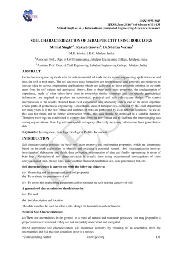
543210–1–2–3–4–5Insertion Loss Stability (dB)Phase Stability ( 020–0.02–0.04–0.06–0.08–0.10051090 Bended Up 290 Bended Left 690 Bended Down 490 Bended Right 8Cable Straight 3Cable Straight 7Cable Straight 5Cable Straight 9 FinalPhase stability vs. frequency.sary or can be fixed mechanically. Guideline VDI/VDE/DGQ/DKD 2622 Part 198 describes one port measurements with the measurement cable connected to a calibrated VNA test port.Rosenberger uses a different method. The measurement cable is connected to the uncalibrated VNA testport and VNA calibration is performed at the free end.This setup is the same as for the intended use and provides some advantages in evaluating the results for transmission stability measurements, since the measurementuncertainty is significantly reduced. This is a benefit forlonger cables and higher frequency bandwidths.Transmission StabilityThe basic setup terminates the free end of the measurement cable with a calibration standard short. Thisputs the measurement cable in the reference positionand uses the VNA trace math to normalize the measuredreturn loss and reflection phase on two different traces.The measurement cable is bent and moved to a different position as needed. The observed change in returnloss and reflection phase must be divided by 2 to obtaininsertion loss stability and phase stability. This is becausethe test signal emitted from the VNA travels through themeasurement cable and is reflected back to the VNA bythe calibration SHORT. It includes twice the cable transmission instabilities. The trace math function and all dataprocessing can alternatively be done on an external PC.Reflection StabilityThe basic setup is to terminate the free end of themeasurement cable with a calibration standard load.This puts the measurement cable in the reference position and uses the VNA trace math, or an external PC, tonormalize the measured return loss. Again, the cable isbent and moved to a different position as needed.Bending ConditionsRosenberger measurement cables are specially designed for use with VNAs and are specified for 90 degrees of bending and relaxation (original position after3x 90 degrees of bending). This is tested in four differentdirections. The 90-degree bending test represents a typical change in cable orientation between a two port VNAcalibration and measurement. Bending procedures used25303540 Fig. 110–120Cable Straight 3Cable Straight 7Cable Straight 5Cable Straight 9 FinalInsertion loss stability vs. frequency. S11 (dB) Fig. 220Frequency (GHz)Frequency (GHz)90 Bended Up 290 Bended Left 690 Bended Down 490 Bended Right 8150510152025303540Frequency (GHz)90 Bended Up 290 Bended Left 690 Bended Down 4 Fig. 490 Bended Right 8Cable Straight 9 Final S11 stability vs. frequency.at Rosenberger are the following:1 90-degree bending test The measurement cable is bent into nine positions and measured: straight,up, straight, down, straight, left, straight, right andstraight. The evaluation starts with the change from oneposition to the next, 1 to 2, 2 to 3 and so on. Exampleresults are shown in Figures 2 through 4.3 90-degree relaxation test The measurementcable is bent into seven positions and measured:straight, up, straight, up, straight, up and straight. Measurements are taken and results are calculated for position 1 and 7. This is repeated for the directions down,left and right.MEASUREMENT EXAMPLETransmission and reflection stability are evaluated fora measurement cable after more than three years of labuse. The solid green and green dashed traces in Figure 2 show bending from the straight position into thedown position and back again to the straight position.The amount of phase change for both sequences is thesame but in opposite directions, as expected. The bluecurves show that the up-direction sequences behavesimilarly but at about half the magnitude.Bending to the right position corresponds to the“natural bending” of the measurement cable and showsthe smallest phase changes. After production, coaxial
ApplicationNotecables typicallyexhibit a “natural–30bending.”The–40coaxial measure–50ment cable hasanon-straight–6005101520form.MeasureFrequency (GHz)(a)ment cables oftenshow best stabil–202440 Frequency Pointsity when bent in–30this direction. For–40the most accurateVNAmeasure–50ment,bending–6005101520in the directionFrequency (GHz)(b)with best stabilityshould be consid Fig. 5 S11 comparison between 305 ered.(a) and 2440 (b) frequency samples.Figure 3 canbe interpreted similarly, although the bending directionwith the worst stability is different.Return loss stability (see Figure 4) is well within specification limits. The bending direction with the worst return loss stability corresponds to the one with the worstphase stability.–20–20–25 S11 (dB)–30MEASUREMENT POINTSThe number of the measurement points is often notincluded in illustrations, test plots or other marketingmaterial; although, without a proper minimum number of measurement points spikes cannot be detected.Spikes are a result of a repeated discontinuities alongthe cable. In VDI/VDE/DGQ/DKD 2622 Part 198 andIEC 60966-1 Chapter 8.1.29, there are formulas to calculate the minimum number of points to detect spikes(see Figures 5 and 6). The measurement of spikes isdescribed in these documents as follows: “cable assemblies might have narrow return loss spikes. Forcontinuous network analyzer systems, the sweep rateshall be low enough and for digital network analyzersystems, the number of measurement points shall behigh enough for resolving eventual return loss spikes.”Figure 6 compares measurements with 305, 610, 1220,2440 and 4880 measurement points. Spikes are visiblebetween 3.7 and 4.2 GHz. Using the formula:cλ (1)f εrεr 1.45 results in a wavelength of 65.6 mm.A half wavelength is 65.2 mm divided by 2 32.8mm. The cable braid in this example is 12 sections witheight strands each. The distance between one full rotation of a section is 28 mm. The velocity factor of thecable results in an electrical length of about 33.7 mm.The reason for the spike is likely a too strongly wrappedcable section (see Figure 7).The minimum number of measurement points is:()n 3 fStop fStart L Cable where:1120(2)–35–40–45–50–55–603.7 S11 (dB) S11 (dB)305 Frequency Points3.83.94.04.14.2Frequency (GHz)RL 305 C2RL 610 C2RL 1220 C2RL 2440 C2RL 4880 C2 Fig. 6 S11 comparison among 305, 610, 1220, 2440 and4880 samples from 3.7 to 4.2 GHz. Fig. 7 Tightly wrapped cable section is the possible causeof a return loss spike.n number of measuring points in the frequencyrange fStart to fStopfStart lowest frequency in the measurement range,in MHzfStop highest frequency in the measurement range,in MHzLCable physical length of the RF measuring cable, inmeters (ignores the relative permittivity εr)The velocity factor is determined by:1Δf 40 k v (3)L CableWhere f is the maximum increment of frequency, inMHz, LCable is the physical length of the RF measuringcable in meters and kv is the velocity factor.CARE AND HANDLING OF CABLE ASSEMBLIESConnector mating is a significant factor influencingperformance. Damaged connectors can also permanentlydamageequipment. Use of agauge is recommended to checkthereferencesof the connectorbefore each measurement (see Figure 8). Center pinprotrusion is critical; if it is too largeit can cause damage and if it is tooshort it can resultin poor electricalperformance. A Fig. 8 Connector gauge.
ApplicationNoteproper torque wrench is necessary for repeatedly reliablecontact without damage. For storage, protection fromsolar radiation, temperature changes and high humidityshould be avoided. A proper storage environment andthe use of protective caps will ensure longevity.Some customers may be familiar with our measurementprotocols. They provide instructions on care and handling,which include important factors to minimize mechanicalstress like adhering to minimum bending radii and avoiding pinching, pulling twisting and free floating.CONCLUSIONCables used for VNA measurements contribute significantly to accuracy and repeatability. RF characteristics like reflection, attenuation and phase length arecritical factors. Test cables should be measured on aregular basis and replaced when they fail to meet specifications. Proper care and handling will be rewardedwith higher accuracy and repeatability. References1. Keysight, “2-Port and 4-Port PNA Network Analyzer,” 71/technicalspecifications/9018-04171.pdf.2.Maury Microwave, “StabilityPlus Microwave/RF Cable Assemblies,” Web: 3. Radiall, “Low Loss High Frequency Flexible Cable Assemblies(SHF Range),” Web: hf-range.html.4. GORE, “VNA Microwave/RF Test Assemblies,” Web: f-test-assemblies.5. Huber Suhner, “Sucoflex 500,” Web: oflex-500.6. Rohde & Schwarz, “R&S ZV-Z9x and R&S ZV-Z19x Test PortCables,” Web: https://cdn.rohde-schwarz.com/pws/dl downloads/dl common library/dl brochures and datasheets/pdf 1/ZV-Z9x ZV-Z19x dat-sw en.pdf.7. Rosenberger, “Test Port Cables & Adaptors,” Web: able-adaptors/.8. “VDI/VDE/DGQ/DKD 2622 Part 19: Calibration of MeasuringEquipment for Electrical Quantities Characterization of HF Measurement Cables,” June 2015.9. “IEC 60966-1: 2019-02, Radio Frequency and Coaxial Cable Assemblies – Part 1: Generic Specification – General Requirementsand Test Methods,” Edition 3, February 2019.
For different branded microwave VNAs there are specifications for the "accuracy of measurements," "typical accuracy" or "uncer-tainty" in tabular and/or graphical form. These values are valid for certain combinations of a VNA type and a calibration kit type and are limited to defined conditions such as source