Transcription
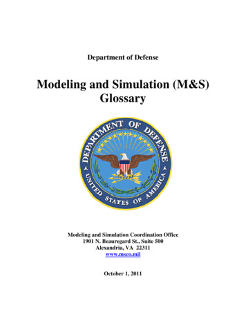
Maxim Design Support Technical Documents Tutorials Wireless and RF APP 5542Keywords: RF, radio frequency, microwave, RF transmitter, digital predistortion, DPD, high-power RF amplifier, CDMA, WCDMA, LTE,frequency domain, X-parameters, time domain, QPSK, QAM, FPGATUTORIAL 5542Modeling and Simulation of RF and Microwave SystemsBy: John Wood, Senior Principal Member of Technical StaffJan 08, 2013Abstract: This application note describes system-level characterization and modeling techniques for radio frequency (RF) and microwavesubsystem components. It illustrates their use in a mixed-signal, mixed-mode system-level simulation. The simulation uses an RF transmitterwith digital predistortion (DPD) as an example system. Details of this complex system and performance data are presented.A similar version of this article appeared in the November/December 2012 issue of IEEE MicrowaveMagazine.IntroductionThe radio frequency (RF) and microwave world has largely been exempt from the rigors of Moore's Law,Click here for an overview of the wirelesswhereas aggressive scaling in the digital world has been the norm for several decades. But now, ascomponents used in a typical radiotransceiver.CMOS transistors have picosecond switching speeds and transition frequencies in the tens to hundredsof GHz, there is an opportunity for the integration of RF and microwave components into a completesystem on a single integrated circuit. Single-chip transceivers for wireless LAN and femtocell basestations are already a commercial reality. As with complex digital systems, the demand for first-pass design success requires that accuratepredictive models are available for the subsystem components of the whole system, enabling the system design to be simulated and anyerrors or faults remedied before the design is committed to hardware. This will save time and the cost of unnecessary fabrication and test ofthe complete system.System-level modeling and simulation for RF and microwave design have become very sophisticated in recent years. Commercial simulationtools with extensive libraries of signal sources, component models, and data analysis tools are now available from EDA vendors such as AWRand Agilent [1, 2]. The development of nonlinear behavioral models for the RF and microwave components such as amplifiers and mixers, andthe ability to measure these subsystems accurately in a typical application environment have been significant enablers of these recentsimulator advances.This tutorial describes the system-level characterization and modeling techniques for RF and microwave subsystem components, andillustrates their use in a mixed-signal, mixed-mode system-level simulation. I shall use an RF transmitter with digital predistortion (DPD) as anexample system, as shown in Figure 1. This is a complex system that includes:RF components such as the power amplifier (PA), for which we need a nonlinear dynamical modelMixed-signal components such as data converters, and IQ modulators/demodulatorsThe digital components of the predistorter, which can be realized as a field-programmable gate array (FPGA) or custom IC, which in turncan be described by models in a high-level description language such as Verilog , or by means of their algorithmic function using amathematical language such as Mathworks' MATLAB software.Page 1 of 10
Figure 1. Block diagram of a wireless infrastructure transmitter system with DPD capability and the observation path for the DPD receiverincluded. This figure shows the major blocks and simulation domains that we shall consider.The RF transmitter with digital predistortion (DPD) is a good example of a practical complex system. Often in such a system, independentteams will design the subsystem components, and yet it is vital to know that the components will work together as a complete system,preferably before the hardware is bolted together. This will allow us to make any necessary architecture changes at the design stage, ratherthan after construction of the hardware.We need a simulation environment that is capable of controlling several different simulator engines and handling the data transfer betweenthem. For example, we may use a harmonic balance or envelope transient simulation for the RF components of the system, whereas thedigital parts of the system will be simulated in a time-stepping or time-marching manner. We may also have to manage floating-point andfixed-point data representations in the different simulators. Having a simulator tool that can manage this cosimulation is essential.Before we get into the details of the models, their construction, and their use in the simulation tools, let's review briefly some of the designchallenges and considerations that we encounter in such a DPD-enabled RF transmitter system. While the design of a high-power RFamplifier to meet the power and efficiency demands of the modern spectrally efficient, digitally modulated communications signals such aswideband CDMA (WCDMA) and long-term evolution (LTE) is challenging enough, the addition of DPD brings an extra wrinkle or two.Modern digitally modulated wireless communications signals such as WCDMA and LTE are designed to maximize the amount of data that canbe transmitted in a given bandwidth. Details of modern wireless communications digital modulation can be found in [3]. Aside from thecomplexity of the modulation and coding schemes, one of the most obvious features of these signals is that they have a very high peak-toaverage power ratio (PAPR), between 6dB and 10dB in practical cases. In other words, the signal peaks can be 10 times higher power thanthe average power of the signal that we want to transmit. The average power determines the range of the transmission; the peak powerdetermines the "size" of the power amplifier. This means that the amplifier must have a power capability four to 10 times that which isnecessary for the base-station coverage area, just to handle the peaks. Running a Class AB PA "backed-off" from its peak capabilitygenerally means running at very low efficiency, which is unacceptable because of the cost of the electricity to run it. Instead, we find highefficiency PA architectures such as the Doherty are used in wireless infrastructure base-station PAs. While efficient, these PAs can producehigh levels of distortion when operated at the high powers necessary. Hence the need for some form of linearization technique, and DPD iscurrently the method of choice.Using DPD brings its own challenges. First, we need to build an observation path (see Figure 1) into the transmitter, to detect the distortionproduced by the PA. The predistorter compares the PA output with the desired signal, and then uses a nonlinear function to generatedistortion in the PA input signal, in such a way that the output of the PA is a replica of the desired signal. The parameters of this nonlinearfunction are continually adapted to minimize the difference between the input signal and the PA output. It's a control system. The predistortercounters the compression characteristic of the PA gain, so it is an expansive function. In the frequency domain, we see that theintermodulation and adjacent channel leakage power is compensated by the DPD. We can think of this as the predistorter adding frequencycomponents to the PA input to counter these distortion products. More details of how the DPD operates can be found in [4].The outcome of adding DPD to the transmitter is that the bandwidth of the predistorted signal is much wider than the original data bandwidth;up to five times wider is a common guideline. This means that the transmit chain from the DPD algorithm, through the DACs and RF section,must be made wide bandwidth. For LTE where carrier aggregation can result in a signal bandwidth of 100MHz, this is a significant design andimplementation challenge. The observation path should also be of this bandwidth to be able to capture the high-order distortion productsproduced by the PA for the DPD system. Further, the observation path needs to be more linear than the rest of the transmitter, as anydistortion introduced here will be indistinguishable from distortion generated by the PA, as far as the DPD is concerned, and the resultingcorrection signal will actually introduce distortion in the PA output. The observation path needs to be low noise and have a high dynamicPage 2 of 10
range to be able to discern the low-level distortion products. These are all significant design challenges, and add to the complexity and cost ofthe transmitter.RF Behavioral ModelsThere has been a considerable body of work produced over the past two decades on the development of behavioral models for nonlinear RFand microwave components [5, 6]. The recent focus is particularly on modeling the PA as this device is the major source of nonlinearity in atypical transmitter system. During this time, the identification of so-called "memory effects" has become one of the foremost challenges inmodeling transmitter systems. While the nonlinearity can be modeled fairly straightforwardly using a polynomial model, for example, theinclusion of memory effects complicates our modeling and simulation task considerably.There are two main approaches to RF behavioral modeling: in the frequency domain, and in the time domain. We will outline both styles. Thenonlinear models are usually based on the linearization of the system-under-test around some operating point, such as the DC condition, orthe average RF power. Anything more general is far too complicated to construct and implement, and doesn't simplify our modeling challenge.Frequency-Domain ModelsThe frequency domain is the natural home for RF and microwave engineers. We have been using S-parameters for linear design for nearly50 years since Kurokawa's original paper [7], and the introduction of the vector network analyzer in the 1960s. Hence, the popularity of thisapproach.A modern and currently popular frequency-domain model is the X-parameters model [8], along with its related and similar model structures,S-functions [9] and the "Cardiff" model [10]. These models are all based on linearization of the nonlinear response around a single large tone—the large signal drive to the PA, for instance. The nonlinear behavior is then probed in the frequency domain by measuring the scatteringresponses to small harmonic signals applied in addition to the large tone. The basic principles and the mathematical underpinnings have beenclearly explained by Verspecht and Root in this magazine [11]. The X-parameters model uses only first-order derivatives to model thenonlinear behavior. This is quite an elegant approach, since the first derivatives are calculated automatically by the simulator in the Jacobianthat it uses for converging to the solution, so this model is simple and fast. The S-functions operate in a similar manner, but can include theDC condition also as an explicit modeling variable. The Cardiff model extends the X-parameters by including higher-order derivatives in themodel, which, like a Taylor Series, extends the region of validity of the model and makes it more general.The value of the X-parameters lies not only in the model formulation, but that the data they are constructed from can be measured using offthe-shelf equipment, such as the Agilent PNA-X nonlinear vector network analyzer. This instrument can also build an X-parameters modelfile that is compatible with the Agilent ADS simulator. High-power PAs do require some extra care in setting up an external measurementsystem around the PNA-X, but this can extend the capability of the instrument to measure X-parameters on PAs of upwards of 100W outputpower [12]. We can also generate an X-parameter description of a circuit from simulation. This means that we can create a nonlinear model ofour circuit or subsystem in a fairly straightforward manner, even quite early on in the design process, for use in a higher-level systemsimulation.One drawback with the X-parameters approach is that these models are memoryless by construction, although there have been recent reportson how to include long- and short-term memory effects into the X-parameters model structure using a Volterra series approach based on theNonlinear Integral Model [13]. The memory effects can be measured using pulsed techniques to observe the transient behavior, and thememory model parameters extracted using NIM methods described in [5], Chapter 3. The memory component is included into the Xparameters formulation through a product term. Since the long-term memory effects are often a result of the bias supply components anddesign of the bias line in the PA fixture, this suggests that it may be possible to model these circuit effects as a separate model componentthat could be "added in" to the X-parameters model of the transistor to yield the complete PA model.Time-Domain ModelsThe natural home for nonlinear dynamical phenomena is the time domain, because we can capture transients, and therefore the energystorage or memory effects, as well as the steady state behavior. A significant historical drawback to using time-domain data for RF andmicrowave circuits is that the sampling rate for measurement must be extremely high, resulting either in undersampling or short time-spandata sets. A similar problem arises in simulation: the time step for transient simulation must be very short, resulting in very long simulationtimes. These problems have nowadays been largely overcome. Recently, real-time sampling oscilloscopes with bandwidth in excess of60GHz, enabling characterization using signals up to 50Gbps have been announced [14]. And the development of envelope transientsimulation techniques has enabled the simulation of circuits using modulated RF and microwave signals in a manageable time.The PAs used in cellular communications are usually quite narrow band, and the output matching network filter attenuates any harmonics.When such PAs are driven into compression, it is the envelope of the signal that is compressed, not the carrier signal, which remainssinusoidal (and may not, in fact, be present explicitly). This means that the nonlinear characteristics of the PA can be completely described bythe envelope behavior. We can use the envelope, or more precisely, the modulation signal to characterize the PA: the timescales for the datacapture are now at the modulation rate. We can also use envelope transient simulation to describe how the modulation signal is affected bythe PA nonlinearities. Thus, our time-domain model of the PA can be constructed at the modulation rate, not at the microwave frequency.The digital modulation used in modern cellular communications is usually created in the form of in-phase (I) and quadrature (Q) components.The I and Q are combined to create the desired modulation signal, usually some form of quadrature phase-shift key (QPSK) or amplitudemodulation (QAM). The time-domain I and Q data can be measured or simulated at the input and output of the PA, and the nonlinear andPage 3 of 10
memory behavior is observed in the AM-to-AM or gain response and the AM-to-PM (phase) response, as shown in Figure 2. What can beseen in these figures are the general trends of gain compression and phase distortion, but also that the responses are in the form of a "cloud"around some average response. It is this cloud that indicates the presence of memory effects. If no memory effects were present, these tworesponses would be single lines—the "instantaneous" response. What the clouds tell us is that the gain at a given output power depends notonly on the input power at that instant, but also on what the value of the signal was at previous times: its history. Not every point in the cloudwill have exactly the same history.Figure 2. AM-to-AM and AM-to-PM plots of the magnitude and phase of the input-output IQ data for a power amplifier. The blue dots are themeasured data, the red dots are the reduced Volterra model predictions.We can build a model of the PA by fitting a curve through the AM-to-AM and AM-to-PM characteristics, using well-known nonlinear data- orfunction-fitting techniques. Essentially we try to fit a known function to the data. Perhaps the most popular and simplest technique is apolynomial fit to the data. In practice, this is usually done using "Least-Squares" methods, which minimize the average Euclidean distancebetween the function and the data. By building the polynomial model, we are basically fitting a Taylor series expansion to the data.But this procedure would yield an instantaneous model, failing to capture the memory effects. We need a model function that includes thehistory of the time domain signal explicitly in its formulation. The Volterra series comes to the rescue. Volterra series can be used to model atime-invariant nonlinear dynamical system; in other words, a nonlinear system with memory. The Volterra series can be thought of as a Taylorseries with memory, and a brief outline is provided in Appendix B: Volterra Series as a Development of a Taylor Series. Since the Volterraseries is related to the Taylor series—both are polynomial functions—then the Volterra series suffers from similar limitations [15]. Primarily,the nonlinearities in the system must not be "strong." In the context of PA modeling, a "strong" nonlinearity would be a discontinuity in theresponse of the input signal, caused by clipping of the waveform, for instance. It is often stated that the (PA) system must be weaklynonlinear for it to be amenable to Volterra analysis: what this means is that the system response must be continuous, and therefore can berepresented by a finite series of contributing terms. Sometimes, "weakly nonlinear" is interpreted as a small number of terms—no more thancubic!—but this is unnecessarily artificial and constrictive.The accuracy of the Volterra series can be improved by increasing the number of terms in the polynomial series. In other words, the model isapproximating the actual data to a smaller tolerance. Whereas increasing the number of terms in a Taylor series is a straightforward exercise,with a Volterra series the cross-terms and memory terms cause the number of terms in the series to increase dramatically as the polynomialdegree and memory depth are increased. This is perhaps one reason why Volterra series modeling has historically seen only limitedapplication. With the computational power now available in modern laptop computers, such limitations on the Volterra series polynomialdegree are a thing of the past.Further, sophisticated "pruning" techniques can be used to limit the number of coefficients in the polynomial to a manageable level, withoutany significant loss of model fidelity. Such techniques were pioneered by Filicori, Ngoya, and coworkers [16, 17], using a technique known asDynamic Deviation. In this method, the Volterra series is expanded explicitly in the deviation of the signal from some operating point, eitherthe DC condition [16] or the average signal power of the PA [17]. Truncating the resulting series to first order in the dynamic deviation wasshown to produce satisfactory results. Unfortunately, rewriting the Volterra series in this way meant that standard least-squares techniques forthe identification of the multinomial coefficients could no longer be used, and so the model parameters were difficult to extract. By recastingthe dynamic deviation expressions, Zhu recovered the linear-in-parameters structure of the Volterra series, enabling straightforward parameterextraction by standard mathematical techniques. This approach also allowed explicit control over the level of dynamics used in the model [18].This technique is known as Dynamic Deviation Reduction, and it can produce accurate power amplifier models with a relatively small numberof coefficients, typically around 30 to 50 being sufficient.The Power Amplifier ModelThe power amplifier is generally the largest contributor to nonlinearity in the transmitter, and the memory effects associated with its frequencyresponse over the wide bandwidth demanded for digital predistortion nowadays require sophisticated nonlinear models to describe the PAbehavior accurately enough for DPD. Typically, a polynomial (Volterra)-based approach is used, although there are notable exceptions to thisin the marketplace. Simple memory-polynomial models used for narrowband signals have been replaced by reduced Volterra series modelsPage 4 of 10
that include some cross-coupling between the memory terms of the series—the cross terms. These models are generally built from thedemodulated IQ data, and hence are baseband models of the RF PA. They are often constructed as a mathematical model in an environmentsuch as MATLAB. The AM-to-AM and AM-to-PM characteristics of a PA and behavioral model are shown in Figure 2. These are plots of themagnitude and phase of the output IQ against the input IQ time-domain data. Such a model can be used easily in a system simulation.Modeling the DPD SystemThe predistortion function is a nonlinear function that compensates the PA gain compression, phase transfer characteristic, and memoryeffects, to produce the linear output from the PA. As noted above, a Volterra-based function is often used in this application.The DPD algorithms for solving the Volterra model are usually developed in a mathematical language such as MATLAB, which affords a richset of tools and functions for solving the nonlinear equations, optimizing the function coefficients, and so forth. Two commonly used DPDapproaches for adaptive linearization are direct adaption and indirect learning, shown schematically in Figure 3. Direct adaption is a classicalcontrol approach; it compares the input signal and (scaled) PA output signal directly and uses the error to drive changes in the DPD functionparameters to minimize the error on the next calculation. Indirect learning is a slightly more complex mathematical process, but can appear tobe easier to implement. Here we compare the predistorted input signal with the postdistorted PA output; we use the same nonlinearpredistortion function. It has been shown mathematically for Volterra series that pre- and post-distortion produce the same behavior, withincertain limits. Again we use the error to drive changes in the predistortion function parameters. This seems easier to implement because theDPD function parameters are used in the calculation of the two signals used for the error (cost) function, and the updated parameters are adirect outcome of the minimization routine.The adaption routine used for estimating the new set of DPD function coefficients is usually a least-squares solver. The least-squaresapproach can be used since the nonlinear Volterra model used for the DPD is set up as a linear-in-parameters expression, as noted earlier.Least-squares minimization routines such as least mean squares (LMS) are often used, and several thousand data (IQ) samples are taken tosolve this over-determined set of equations. The LMS routine is generally quite stable, though it can be slow to converge. More aggressiveminimization techniques such as recursive least squares (RLS) and affine projection (AP) have been demonstrated [19], offering fasterconvergence, although they can be more prone to instability arising from noise in the input data. This can be overcome with care in theimplementation.Figure 3. Schematic representations of DPD functions: (a) is adaptive control, (b) is indirect learning.Once the DPD algorithms have been demonstrated in the MATLAB environment, the DPD model can then be imported into the systemsimulator, and the linearization of the PA in a more complex, multisimulator environment can be simulated. After the system performance hasbeen verified, the MATLAB model code can then be downloaded directly into an FPGA using development software provided by FPGAmanufacturers such as Xilinx and Altera. The mathematical model can then be run in hardware, in real time, and any practical implementationerrors can be addressed quickly.Page 5 of 10
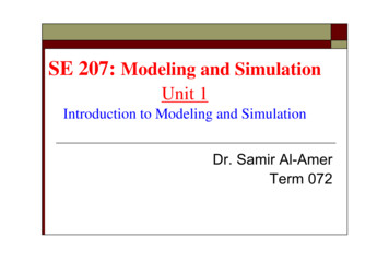
Mixed-Signal Models and SimulationWe are now left with modeling and simulating the "glue" circuits that connect the digital pieces—the predistorter—to the RF power amplifier.Often, these circuits and components are omitted from the system specification, with the verification of the linearized performance focusingonly on the PA and DPD models. But actually, these components do rather more than act as glue. As we mentioned earlier, the DPDobservation path is a critical component of this linearized transmitter system, and its performance can have major impact on the overalloperation and capability of the transmitter.With suitable models for the data converters, modulators and demodulators (mod/demod), and the RF components such as driver and lownoise amplifiers, we can simulate the behavior of the complete transmitter in detail. We can use the simulation to study the impact of thesecomponents' specifications on the overall performance of the linearized transmitter. For example, we can study the effects of the phase noiseperformance of the local oscillator in the mod/demod circuit on the accuracy and dynamic range of the observation path, and hence test thelimits of the linearization capability of the complete system. The models that we choose for these components and circuits will depend largelyon how sophisticated we want the simulated behavior to be, and how important the impairments are to the linearized.The Data ConvertersModels for the digital-to-analog converters (DACs) and analog-to-digital converters (ADCs) range from simple input/output models, throughVerilog descriptions of the functional behavior, to sophisticated nonlinear models that approach (or even exceed) the complexity of the PAnonlinear models. The data converters are nonlinear devices. At a high level, the nonlinearity can be modeled as harmonic generation in thefrequency domain. More sophisticated models will use a polynomial or Volterra approach. At the system-level description for the transmitter, itmay be sufficient to include a simple nonlinearity and the noise figure, particularly for the ADC in the observation path, to model andinvestigate the limitations on the linearization capability arising from low distortion signal powers.System-level simulation tools such as Agilent's SystemVue and AWR's Virtual System Simulator (VSS) come with built-in models for manycommercial data converters. While this is useful for verification of the final system, using the more generic data-converter models available inthese tools allows us to investigate some of the more straightforward limitations of these components, such as the number of data bits, noisefigure, clock frequency and frequency response, and so forth. These investigations can give us a better understanding of the nature of thelimitations of these factors or impairments on the overall system performance.The IQ Modulator/Demodulator CircuitsIn our simulation, we can use ideal models for the IQ modulation and demodulation functions, or analog circuit descriptions or macromodelsthat include many physical behaviors that contribute to the performance, and performance limitations of these devices. Our main concerns arelikely to be the impacts of these impairments to ideal demodulator behavior on the performance of the observation path. Such impairmentsinclude the injection of noise from the local oscillator (LO), so the LO phase noise performance is of interest, and the introduction of cross-talkbetween the I and Q paths in the demodulator.These IQ demodulator imperfections can be modeled using a simple analytical circuit model described by Cavers [20] and shown in Figure 4.The output from the ideal demodulator, which is usually available as a built-in model in the RF or system-level simulator, is fed through thetwo linear amplifiers, allowing a gain imbalance to be modeled. The phase imbalance, Φ, or the difference from quadrature phase between theI and Q paths, is modeled using the cross talk and in-line amplifiers in sin(Φ) and cos(Φ), respectively. The output of this analytical modelenables the inclusion of DC offsets into the output of the modulator. This is important for zero-IF downconversion architectures.Figure 4. Analytical circuit model for IQ demodulator impairments.The RF Amplifiers and FiltersThe PA driver amplifiers in the transmit path are usually not driven too hard, so their nonlinear behavior is less of a concern than that of thePA itself. This means that we can use either simpler behavioral models for these components, or the nonlinear models that are provided bythe component vendors for use in the RF circuit simulator. These models should be checked that they can be used in a transient simulationbefore we use them, though, since the system simulation will use a time-stepping (transient) algorithm. Any distortion produced by the driveramplifiers' nonlinearities will be included in the net output from the PA, and will in practice be accommodated by the predistorter. Our mainconcern in the system-level simulation is that these nonlinearities are captured sufficiently well and that their impact on the overall nonlinearbehavior of the transmitter is described. As noted above, the major source of nonlinear behavior is the PA itself. Therefore, it is mostimportant that the PA's nonlinear dynamical behavior is properly described.Page 6 of 10
The low-noise amplifier (LNA) in the observation path plays an important role in determining the noise level or sensitivity of the predistortionsystem. Again, it is usually sufficient to use a system-level model available in the system or RF simulator, and adjust the gain, noise figure,and frequency response of this component, to understand and ultimately control the contributions of these performance specifications on theoverall performance of the linearized system.The transmit and o
This tutorial describes the system-level characterization and modeling techniques for RF and microwave subsystem components, and illustrates their use in a mixed-signal, mixed-mode system-level simulation. I shall use an RF transmitter with digital predistortion (DPD) as an example system, as shown in Figure 1. This is a complex system that .