WIXLIB

each iteration estimates the largest Fourier coefficient(the one least impacted by leakage) and subtracts itscontribution to the time signal. The iterative update ofthe time signal causes a large increase in runtime. Thealgorithms in [GGI 02, Man92] perform this update bygoing through O(k) iterations each of which updatesat least O(k) time samples, resulting in an O(k 2 ) termin the runtime. The algorithm [GMS05], introduceda ”bulk sampling” algorithm that amortizes this process but it requires solving instances of a non-uniformFourier transform, which is expensive in practice.Interpolation-based algorithms are less commonand limited to the design in [Iwe10a]. This approachuses a leakage-free filter, G, to avoid the need for iteration. Specifically, the algorithm in [Iwe10a] uses for G afilter in which Gi 1 iff i mod n/p 0 and Gi 0 otherwise. The Fourier transform of this filter is a “spiketrain” with period p. This filter does not leak: it is equalto 1 on 1/p fraction of coordinates and is zero elsewhere.Unfortunately, however, such a filter requires that p divides n; moreover, the algorithm needs several differentvalues of p. Since in general one cannot assume that nis divisible by all numbers p, the algorithm treats thesignal as a continuous function and interpolates it atthe required points. Interpolation introduces additionalcomplexity and increases the exponents in the runtime.Our approach. The key feature of our algorithmis the use of a different type of filter. In the simplestcase, we use a filter obtained by convolving a Gaussianfunction with a box-car function. A more efficient filtercan be obtained by replacing the Gaussian functionwith a Dolph-Chebyshev function. (See Fig. 1 for anillustration.)Because of this new filter, our algorithm does notneed to either iterate or interpolate. Specifically, thefrequency response of our filter Ĝ is nearly flat insidethe pass region and has an exponential tail outsideit. This means that leakage from frequencies in otherbuckets is negligible, and hence, our algorithm neednot iterate. Also, filtering can be performed using theexisting input samples xi , and hence our algorithm neednot interpolate the signal at new points. Avoiding bothiteration and interpolation is the key feature that makesour algorithm efficient.Further, once a large coefficient is isolated in abucket, one needs to identify its frequency. In contrastto past work which typically uses binary search for thistask, we adopt an idea from [PS10] and tailor it toour problem. Specifically, we simply select the set of“large” bins which are likely to contain large coefficients,and directly estimate all frequencies in those bins. Tobalance the cost of the bin selection and estimationsteps, we make the number of bins somewhat larger thanthe typical value of O(k). Specifically, we use B which leads to the stated runtime. 62 nk,NotationTransform-Related Notations. For an inputsignal x Cn , its Fourier spectrum is denoted by x̂.We will use x y to denote the convolution of x and y,and x · y to denote the coordinate-wise product of x and2πi/ny. Recall that xd· y x̂ ŷ. We define ωto be ea primitive nth root of unity (here i 1, but in therest of the paper, i is an index).Indices-Related Notations. All operations onindices in this paper are taken modulo n. Thereforewe might refer to an n-dimensional vector as havingcoordinates {0, 1, . . . , n 1} or {0, 1, . . . , n/2, n/2 1, . . . , 1}. interchangeably. Finally, [s] refers to the setof indices {0, . . . , s 1}, whereas supp(x) refers to thesupport of vector x, i.e., the set of non-zero coordinates.In this paper we assume that n is an integer powerof 2.3Basics(a) Window Functions. In digital signal processing [OSB99] one defines window functions in thefollowing manner:Definition 3.1. We define a ( , δ, w) standard window function to be a symmetric vector F Rn withsupp(F ) [ w/2, w/2] such that F̂0 1, F̂i 0 for alli [ n, n], and F̂i δ for all i / [ n, n].Claim 3.2. For any and δ, there exists an( , δ, O( 1 log(1/δ))) standard window function.Proof. This is a well known fact [Smi11]. For example, for any and δ, one can obtain a standard windowp by taking a Gaussian with standard deviation Θ( log(1/δ)/ ) and truncating it at w O( 1 log(1/δ))). The Dolph-Chebyshev window functionalso has the claimed property but with minimal big-Ohconstant [Smi11] (in particular, half the constant of thetruncated Gaussian). The above definition shows that a standard windowfunction acts like a filter, allowing us to focus on a subsetof the Fourier coefficients. Ideally, however, we wouldlike the pass region of our filter to be as flat as possible.6 Although it is plausible that one could combine our filterswith the binary search technique of [GMS05] and achieve analgorithm with a O(k logc n) runtime, our preliminary analysisindicates that the resulting algorithm would be slower. Intuitively,observe that for n 222 and k 211 , the values of nk 216.5 92681 and k log2 n 45056 are quite close to each other.

Definition 3.3. We define a ( , 0 , δ, w) flat window Lemma 3.6. If j 6 0, n is a power of two, and σ isfunction to be a symmetric vector F Rn with a uniformly random odd number in [n], then Pr[σj supp(F ) [ w/2, w/2] such that F̂i [1 δ, 1 δ] [ C, C]] 4C/n.for all i [ 0 n, 0 n] and F̂i δ for all i / [ n, n].Proof. If j a2b for some odd a, then the orbit of σj isA flat window function (like the one in Fig. 1) can be ob- a0 2b for all odd a0 . There are thus 2 · round(C/2b 1 ) tained from a standard window function by convolving 4C/2b 1 possible values in [ C, C] out of n/2b 1 suchit with a “box car” window function, i.e., an interval. elements in the orbit, for a chance of at most 4C/n. Specifically, we have the following.Note that for simplicity, we will only analyze ourClaim 3.4. For any , 0 , and δ with 0 , there exists algorithm when n is a power of two. For general n,n1an ( , 0 , δ, O( 0 log δ )) flat window function.the analog of Lemma 3.6 would lose an n/ϕ(n) O(1) O(log log n) factor, where ϕ is Euler’s totient function.Note that in our applications we have δ 1/nThis will correspondingly increase the running time ofand 2 0 . Thus the window lengths w of the flatthe algorithm on general n.window function and the standard window function areClaim 3.5 allows us to change the set of coeffithe same up to a constant factor.cients binned to a bucket by changing the permutation;Proof. Let f ( 0 )/2, and let F be an Lemma 3.6 bounds the probability of non-zero coeffiδ, w) standard window function with minimal cients falling into the same bucket.(f, ( 0 )n(c) Subsampled FFT. Suppose we have a vector( 0 )n2w O( ). We can assume , 0 1/(2n)0 logδx Cn and a parameter B dividing n, and would like0(because [ n, n] {0} otherwise), so log ( δ )n to compute ŷi x̂i(n/B) for i [B].O(log nδ ). Let Fˆ0 be the sum of 1 2( 0 f )n adjacentClaim 3.7. ŷ is the B-dimensional Fourier transformPn/B 1copies of F̂ , normalized to Fˆ0 0 1. That is, we defineof yi j 0 xi Bj .P( 0 f )nTherefore ŷ can be computed in O( supp(x) j ( 0 f )n F̂i j0ˆBlogB) time.F i Pf nF̂jj f nProof.so by the shift theorem, in the time domainB 1n 1X n/B 1XX( 0 f )nij(n/B)XxBj a ω i(Bj a)n/Bxω x̂ ji(n/B)0jFa Faω .a 0 j 0j 0j ( 0 f )nSince F̂i 0 for i f n, the normalization factorPf n00j f n F̂j is at least 1. For each i [ n, n], thesum on top contains all the terms from the sum onbottom. The other 2 0 n terms in the top sum havemagnitude at most δ/(( 0 )n) δ/(2( 0 f )n), so Fˆ0 i 1 2 0 n(δ/(2( 0 f )n)) δ. For i n,however, Fˆ0 i 2( 0 f )nδ/(2( 0 f )n) δ. Thus F 0is an ( , 0 , δ, w) flat window function, with the correctw. B 1X n/B 1Xa 0j 0as desired.4xBj a ω ian/B B 1Xya ω ian/B ŷi ,a 0 AlgorithmA key element of our algorithm is the inner loop,which finds and estimates each “large” coefficient withconstant probability. In §4.1 we describe the inner loop,and in §4.2 we show how to use it to construct the full(b)Permutation of Spectra. Following algorithm.[GMS05], we can permute the Fourier spectrum as fol4.1 Inner Loop Let B be a parameter that dilows by permuting the time domain:vides n, to be determined later.Let G be aClaim 3.5. Define the transform Pσ,τ such that, given (1/B, 1/(2B), δ, w) flat window function for some δ andan n-dimensional vector x, an integer σ that is invertible w O(B log n ). We will have δ 1/nc , so one canδmod n, and an integer τ [n], (Pσ,τ x)i xσi τ . Then think of it as negligiblysmall. τ i\(P.There are two versions of the inner loop: locationσ,τ x)σi x̂i ωloops and estimation loops. Location loops are givenPnaj\Proof. For all a, (P a parameter d, and output a set I [n] of dkn/Bσ,τ x)aj 1 xσj τ ωPn 1a(j τ )σ 1 x̂aσ 1 ω τ aσ . coordinates that contains each large coefficient withj 1 xj ω

G (linear scale)b (linear 0150200(a)(b)G (log scale)b (log 0100150200250(d)Figure 1: An example flat window function for n 256. This is the sum of 31 adjacent (1/22, 10 8 , 133)Dolph-Chebyshev window functions, giving a (0.11, 0.06, 2 10 9 , 133) flat window function (although our proofb in a linearonly guarantees a tolerance δ 29 10 8 , the actual tolerance is better). The top row shows G and Gscale, and the bottom row shows the same with a log scale.

“good” probability. Estimation loops are given a set We have thatI [n] and estimate xI such that each coordinate isn 1Xestimated well with “good” probability.\ ŷσi oσ (i) 2 (Pσ,τ x)t Ĝσi t oσ (i)2t 01. Choose a random σ, τ [n] with σ odd.2. Define y G · (Pσ,τ x), so yi Gi xσi τ . Thensupp(y) supp(G) [w].3. Compute ẑi ŷi(n/B) for i [B]. By Claim 3.7,Pdw/Be 1this is the DFT of zi j 0yi jB .4. Define the “hash function” hσ : [n] [B]by hσ (i) round(σiB/n) and the “offset”oσ : [n] [ n/(2B), n/(2B)] by oσ (i) σi hσ (i)(n/B).5. Location loops: let J contain the dk coordinatesof maximum magnitude in ẑ. Output I {i [n] hσ (i) J}, which has size dkn/B.6. Estimation loops: for i I, estimate x̂i asx̂0i ẑhσ (i) ω τ i /Ĝoσ (i) .By Claim 3.7, we can compute ẑ in O(w B log B) O(B log nδ ) time. Location loops thus take O(B log nδ dkn/B) time and estimation loops take O(B log nδ I )time. Fig. 2 illustrates the inner loop.For estimation loops, we get the following guarantee: 2n 1X\(Pσ,τ x)σj Ĝσ(i j) oσ (i)j 02 2X\(Pσ,τ x)σj Ĝσ(i j) oσ (i)j T2 2X\(Pσ,τ x)σj Ĝσ(i j) oσ (i)j T/22 2(1 δ)XPr [ x̂0i x̂i 2 σ,τk 22kx̂ S k2 3δ 2 kx̂k1 ] O( ).k B 2δ\(Pσ,τ x)σjj TX\(Pσ,τ x)σjj T/In the last step, the left term follows from Ĝa 1 δ for all a. The right term is because for j /T , σ(i j) oσ (i) σ(i j) oσ (i) 2n/B n/(2B) n/B, and Ĝa δ for a n/B. ByClaim 3.5, this becomes:22Lemma 4.1. Let S be the support of the largest kcoefficients of x̂, and x̂ S contain the rest. Then forany 1,22X2 ŷσi oσ (i) 2(1 δ)x̂j ω τ j2 2δ 2 kx̂k1 .j T2P τ jDefine V . As a choice over τ ,j T x̂j ωV is the energy of a random Fourier coefficient of thevector x̂T so we can bound the expectation over τ :2E[V ] kx̂T k2 .Proof. By the definitions,x̂0i ẑhσ (i) ω τ i /Ĝoσ (i) ŷσi oσ (i) ω τ i /Ĝoσ (i) .τNow, for each coordinate j 6 i, Prσ [j T ] 8/B byLemma 3.6. Thus Prσ [S T 6 ] 8k/B, so withprobability 1 8k/B over σ we haveConsider the case that x̂ is zero everywhere but at i,\so supp(Pσ,τ x) {σi}. Then ŷ is the convolution of Ĝ\and Pσ,τ x, and Ĝ is symmetric, so\\ŷσi oσ (i) (Ĝ Pσ,τ x)σi oσ (i) Ĝ oσ (i) Pσ,τ xσi Ĝoσ (i) x̂i ω τ i2kx̂T k2 x̂T \S22.Let E be the event that this occurs, so E is 0 withprobability 8k/B and 1 otherwise. We have2E [EV ] E[E kx̂T k2 ] E[E x̂T \Sσ,τσσ2]2 E[ x̂T \Sσ2].2which shows that x̂0i x̂i in this case. But x̂0i x̂i is Furthermore, we knowlinear in x̂, so in general we can assume x̂i 0 andX2bound x̂0i .E [EV ] E[ x̂T \S 2 ] x̂j 2 Pr[σ(i j) [ 2n/B, 2n/B]]σ,τσσ0Since x̂i ẑhσ (i) /Ĝoσ (i) ẑhσ (i) /(1 δ) j S/ ŷσi oσ (i) /(1 δ), it is sufficient to bound ŷσi oσ (i) .82 kx̂ S k2Define T {j [n] σ(i j) [ 2n/B, 2n/B]}.B

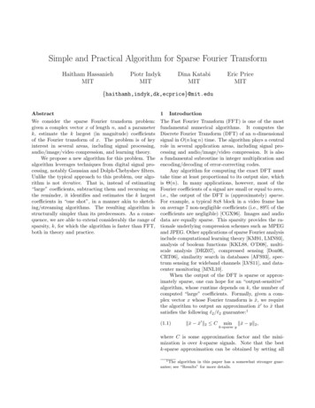
Convolved signal10.80.60.40.20MagnitudeMagnitudePermuted deMagnitudeRegions estimated 3π/2ŷ G\· Pσ,τ xChosen region\Pσ,τ xẑSample cutoffẑ(c)2π(b)Samples actually computedπ/23π/2\Pσ,τ x\ŷ G · Pσ,τ x\Pσ,τ x0π2π(d)Figure 2: Example inner loop of the algorithm on sparse input. This run has parameters n 256, k 4,G being the (0.11, 0.06, 2 10 9 , 133) flat window function in Fig. 1, and selecting the top 4 of B 16 samples.In part (a), the algorithm begins with time domain access to Pσ,τ x given by (Pσ,τ x)i xσi τ , which permutesthe spectrum of x by permuting the samples in the time domain. In part (b), the algorithm computes the timedomain signal y G · Pσ,τ x. The spectrum of y (pictured) is large around the large coordinates of Pσ,τ x. Thealgorithm then computes ẑ, which is the rate B subsampling of ŷ as pictured in part (c). During estimation loops,the algorithm estimates x̂i based on the value of the nearest coordinate in ẑ, namely ẑhσ (i) . During location loops(part (d)), the algorithm chooses J, the top dk (here, 4) coordinates of ẑ, and selects the elements of [n] thatare closest to those coordinates (the shaded region of the picture). It outputs the set I of preimages of thoseelements. In this example, the two coordinates on the left landed too close in the permutation and form a “hashcollision”. As a result, the algorithm misses the second from the left coordinate in its output. Our guarantee isthat each large coordinate has a low probability of being missed if we select the top O(k) samples.

by Lemma 3.6. Therefore, by Markov’s inequality and and by Lemma 4.1,a union bound, we have for any C 0 thatknE[ V ] O( ).C B2Pr [V 8 kx̂ S k2 ] Pr [E 0 EV C E [EV ]]σ,τσ,τσ,τB1n] O( d),Thus by Markov’s inequality Pr[ V dk Bkor 8 1/C.Bn1Pr[ U V dk k(1 1/ )] O( ).HenceB dC22(1 δ)2 kx̂ S k2 2δ 2 kx̂k1 ]Bk 8 1/C.BPr [ ŷσi oσ (i) 2 16σ,τSince the RHS is only meaningful for d 1/ we haven k(1 1/ ). Thereforedk BPr[ U V dkn1] O( ).B dReplacing C with B/(32k) and using x̂0i x̂i and thus ŷσi oσ (i) /(1 δ) gives1Pr[ {j [B] ẑj 3(1 δ)E} kd] O( ). d2 2 1 δ 222() kx̂ S k2 δ kx̂k1 ]Pr [ x̂0i x̂i 2 σ,τ2k 1 δ1 δHence a union bound over this and the probability thatk x̂0i x̂i E gives (8 32/ ) .Bk1Pr[i / I] O( )which implies the result. B dFurthermore, since Ĝoσ (i) [1 δ, 1 δ], ẑhσ (i) is a good estimate for x̂i —the division is mainly usefulfor fixing the phase. Therefore in location loops, we getthe following guarantee:q22 2Lemma 4.2. Define E k kx̂ S k2 3δ kx̂k1 to bethe error tolerated in Lemma 4.1. Then for any i [n]with x̂i 4E,Pr[i / I] O(k1 ) B das desired. 4.2 Outer Loop Our algorithm is parameterized by and δ. It runs L O(log n)qiterations of the innerloop, with parameters B O(nk log(n/δ) )7and d O(1/ ) as well as δ.1. For r {1, . . . , L}, run a location inner loop toget Ir .2. For each i I I1 · · · IL , let si {r i Ir } .3. Let I 0 {i I si L/2}.4. For r {1, . . . , L}, run an estimation inner loopon I 0 to get x̂rI 0 .5. For i I 0 , estimate x̂0i median({x̂ri i I 0 }),where we take the median in real and imaginarycoordinates separately.kProof. With probability at least 1 O( B), x̂0i x̂i E 3E. In this case ẑhσ (i) 3(1 δ)E.Thus it is sufficient to show that, with probability at1least 1 O( d), there are at most dk locations j [B]with ẑj 3(1 δ)E. Since each ẑj corresponds ton/B locations in [n], we will show that with probability1at least 1 O( d), there are at most dkn/B locations Lemma 4.3. Thealgorithmrunsinqj [n] with x̂0j 3(1 δ)2 E.nk log(n/δ)log n).O( Let U {j [n] x̂j E}, and V {j [n] x̂0j x̂j E}. Therefore {j [n] x̂0j 2E} U V .Proof. To analyze this algorithm, note thatSince 2 3(1 δ)2 , we haveXL X I 0 si Ir Ldkn/B{j x̂0j 3(1 δ)2 E} U V .2ritimeWe also know U k 2kx S k2E27 Note k(1 1/ )that B is chosen in order to minimize the running time.For the purpose of correctness, it suffices that B ck/ for someconstant c. We will use this fact later in the experimental section.

or I 0 2dkn/B. Therefore the running time of boththe location and estimation inner loops is O(B log nδ dkn/B). Computing I 0 and computing the mediansboth take linear time, namely O(Ldkn/B). Thus thetotal running time is O(LB log nδ Ldkn/B). Pluggingqnkin B O( log(n/δ)) and d O(1/ ), this runningqtime is O( nk log(n/δ)log n). We require B Ω(k/ ), however; for k n/ log(n/δ), this would cause the runtime to be larger. But in this case, the predicted runtime is Ω(n log n) already, so the standard FFT is fasterand we can fall back on it. all i / I 0 have x̂0i 0 and x̂i 4E with probability1 1/n2 , with total probability 1 2/n2 we have2kx̂0 x̂k 16E 2 16 22kx̂ S k2 48δ 2 kx̂k1 .kRescaling and δ gives our theorem.5 Experimental Evaluation5.1 Implementation We implement our algorithmin C using the Standard Template Library, andrefer to this implementation as sFFT (which stands for“sparse FFT”). We have two versions: sFFT 1.0, whichTheorem 4.4. Running the algorithm with parameters implements the algorithm as in §4, and sFFT 2.0, whichadds a heuristic to improve the runtime. , δ 1 gives x̂0 satisfyingsFFT 2.0. The idea of the heuristic is to apply 22220thefilterused in [Man92] to restrict the locations of thekx̂ x̂k kx̂ S k2 δ kx̂k1 .klarge coefficients. The heuristic is parameterized by anM dividing n. During a preprocessing stage, it does thewithq probability 1 1/n and running time following:log n).O( nk log(n/δ) 1. Choose τ [n] uniformly at random.Proof. Define2. For i [M ], set yi xi(n/M ) τ .3. Compute ŷ.r 224. Output T [M ] containing the 2k largestkx̂ S k2 3δ 2 kx̂k1E kelements of ŷ.Lemma 4.2 says that in each location iteration r, for Observe that ŷ Pn/M x̂ τ (i M j). Thus,iM j i ωj 0any i with x̂i 4E,XE[ ŷi 2 ] x̂j 2 .k1rτPr[i / I ] O( ) 1/4.i j mod M B dThus E[si ] 3L/4, and each iteration is an independenttrial, so by a Chernoff bound the chance that si L/2is at most 1/2Ω(L) 1/n3 . Therefore by a union bound,with probability at least 1 1/n2 , i I 0 for all i with x̂i 4E.Next, Lemma 4.1 says that for each estimationiteration r and index i,Pr[ x̂ri x̂i E] O(k) 1/4. BTherefore, with probability 1 2 Ω(L) 1 1/n3 , x̂ri x̂i E in at least 2L/3 of the iterations.Since real(x̂0i ) is the median of the real(x̂ri ), theremust exist two r with x̂ri x̂i E but one real(x̂ri )above real(x̂0i ) and one below. Hence one of these r has real(x̂0i x̂i ) real(x̂ri x̂i ) E, and similarly forthe imaginary axis. Then x̂0i x̂i 2 max( real(x̂0i x̂i ) , imag(x̂0i x̂i ) ) 2E.By a union bound over I 0 , with probability at least1 1/n2 we have x̂0i x̂i 2E for all i I 0 . SinceThis means that the filter is very efficient, in that ithas no leakage at all. Also, it is simple to compute.Unfortunately, it cannot be “randomized” using Pσ,τ :after permuting by σ, any two colliding elements j andj 0 (i.e., such that j j 0 (mod M )) continue to collide.Nevertheless, if x̂j is large, then j (mod M ) is likely tolie in T —at least heuristically on random input.sFFT 2.0 completes the algorithm assuming that all“large” coefficients j have j mod M in T . That is, inthe main algorithm of §4, we then restrict our sets Ir tocontain only coordinates i with (i mod M ) T . Weexpect that Ir 2kM dkn/B rather than the previousdkn/B. This means that our heuristic will improve theruntime of the inner loops from O(B log(n/δ) dkn/B)kto O(B log(n/δ) Mdkn/B M dk), at the cost ofO(M log M ) preprocessing.Note that on worst case input, sFFT 2.0 may giveincorrect output with high probability. For example, ifxi 1 when i is a multiple of n/M and 0 otherwise,then y 0 with probability 1 M/n and the algorithmwill output 0 over supp(x). However, in practice thealgorithm works for ”sufficiently random” x.

Claim 5.1. As a heuristic approximation, sFFT 2.0Experimental Setup. The test signals are generruns in O((k 2 n log(n/δ)/ )1/3 log n) as long as k ated in a manner similar to that in [IGS07]. For the run 2 n log(n/δ).time experiments, k frequencies are selected uniformlyat random from [n] and assigned a magnitude of 1 andJustification. First we will show that the heuristic a uniformly random phase. The rest are set to zero.improves the inner loop running time to O(B log(n/δ) For the tolerance to noise experiments, the test signalskare generated as before but they are combined with adM dkn/B M dk), then optimize the parameters Mand B.ditive white Gaussian noise, whose variance varies deHeuristically, one would expect each of the Ir to be a pending on the desired SNR. Each point in the graphs T M factor smaller than if we did not require the elements is the average over 100 runs with different instances ofto lie in T modulo M . Hence, we expect each of the Ir test signals and different instances of noise. In all ex kperi

algorithms and their complex structures limit their ap-plicability to only very sparse signals. In particular, the more recent algorithms were implemented and evaluated empirically against FFTW, an e cient implementation of the FFT with a runtime O(nlogn) [Iwe10a, IGS07]. The results show that the algorithm in [GMS05] is com-