Transcription
Optimal design of elastic columns formaximum buckling loadDragan T. SpasićUniversity of Novi Sad, YugoslaviaE-mail: spasic@uns.ns.ac.yuAbstractThe problem of Lagrange, to nd the curve which by its revolution about an axisin its plane determines the column of greatest e ciency, is examined. A comparisonis made between the optimal shapes of the compressed column predicted by severalexisting formulations for columns of circular cross section hinged at the end points.Then, two di erent generalizations of the problem, that follow from a generalizedplane elastica and the theory called Kirchho ’s kinetic analogue, are considered.The optimal shape of a compressed column that can su er not only ‡exure as inclassical elastica theory, but also compression and shear is rst presented. Second,the distribution of material along the length of a compressed and twisted columnis optimized so that the column is of minimum volume and will support a givenload without spatial buckling. Necessary conditions for both problems are derivedusing the maximum principle of Pontryagin. The optimal shapes are obtained bynumerical integration. The principal novelty of the present results is that bothsolutions, that follow from two possible generalizations of the classical BernoulliEuler bending theory, lead to the optimum column with non-zero cross sectionalarea at its ends.1IntroductionThe problem of determining that shape of compressed column which has the largest Eulerbuckling load was posed by Lagrange in 1773. Clausen in 1851 solved it for columns ofcircular cross section pined at the end points. Although that result was mathematicallycorrect the obtained optimal shape did have points where the cross section vanishes.Nikolai [1], in work long unnoticed outside the Soviet Union, was the rst author whoconsidered that anomaly of Clausen’s solution. In order to avoid any nite load to inducein nite stresses in the column, Nikolai proposed minimal cross sectional area at the ends,determined so that given limiting stress will not be exceeded. Since then, many results ofstructural optimization could be related to the problem of Lagrange. Mathematically, thisamounts to maximizing an eigenvalue of a certain Sturm-Liouville system to obtain anisoperimetric inequality. It is worth noting that the problem of Lagrange with clampedclamped boundary conditions, was attacked in 1962 by Tadjbakhsh and Keller [2] in thecontinuation of work Keller [3] had begun at the suggestion of Cli ord Truesdell. That
case, in which the column is clamped at each end, seems to be especially troublesomesince the solution has two points in its interior where the cross sections vanishes.It is obvious that these extremal shapes have led to confusion and several attemptsto resolve the anomaly. Nearly in the same manner as Nikolai, Trahair and Booker [4]have considered the problem of avoiding the zero cross sectional area at the end of theoptimal column. In 1977 Olho and Rasmussen [5] noted what’s wrong in Tadjbakhshand Keller’s work. Also they presented bimodal formulation of the column problem.Namely, structural optimization combines mathematics and mechanics with engineeringand has become a broad multidisciplinary eld, see Prager and Taylor [6], Rozvany andMroz [7] and Vanderplaats [8]. The constant ‡ow of general reviews, surveys of sub eldsand conference proceedings on optimal design testify the strong activity and increasingimportance of the eld, see Olho and Taylor [9] as a source for additional bibliography.We note that the problem of Lagrange and the optimal shapes for which the cross sectionsvanishes at certain points were reconsidered many times, see results of Barnes [10], [11],Seiranian [12], Plaut et al. [13] and Cox and Overton [14]. Now it is clear that all theseresults are mathematically correct. Also it is remarkable that these results were based onthe linear equilibrium equations that follow from Bernoulli-Euler bending theory as thesimplest model for the planar ‡exure of an elastic column described by an inextensiblecurve constrained to lie in plane.Optimization of columns for maximum buckling load still remains a topic of widespread interest. In what follows, the problem of Lagrange is generalized in two directions.First, the optimal shape of compressed column that can su er not only ‡exure as in theclassical elastica theory, but also compression and shear will be considered. Also, byuse of Kirchho ’s kinetic analogue, see Antman and Kenney [15], the optimal shape ofcompressed and twisted column against spatial buckling will be determined. We shallshow that both solutions that follow from these two possible generalizations of the classical Bernoulli-Euler elastica theory lead to the optimum columns with non-zero crosssectional area at the ends. Namely, according to Clausen’s solution the optimum columnhas zero cross sectional area at the ends, and therefore, roughly speaking, at the ends doesnot recognize the di erence between any applied nite load and, for example, its doubledvalue. It seems that Clausen’s solution will never t for real columns. In consideringNikolai’s work [1] and his comments on that solution, three points should be noted. First,the condition that limiting stress should be included in the column problem is taken fromthe linear theory called strength of materials. Secondly, it was implicitly allowed thatthe strongest column will change its length under compression. Thus, Nikolai’s solutioncould not be considered within Bernoulli-Euler beam theory because the classical theoryof buckling neglects axial strain of the central line as a possible deformation of an elastic rod. Lastly, although according to Gjelsvik [16], the rst work that generalizes theclassical elastica theory as to take the shearing forces into account goes back to Engesser,who considered the in‡uence of shear on the buckling loads in 1889, in the problem ofLagrange the in nite value of shear rigidity was assumed.The aim of any theory of rods or beams is to describe the deformed con gurationof a slender three-dimensional body by a single curve and certain parameters recordingmaterial orientation relative to that curve, see Parker [17]. The three-dimensional elasticconstitutive law is replaced by expressions for resultant forces, moments and generalized
moments in terms of extension, curvatures, torsion and the remaining parameters. Eachresulting theory must necessarily be approximate, although its accuracy should increaseas the representative scale of distance along the axis of the rod increases relative to atypical diameter of the cross section. According to that lines we nd that Clausen’ssolution is correct in sense of the classical Bernoulli-Euler elastica theory, and if we wouldlike to improve it to t for real columns we are to pose the column problem within ageneralized plane elastica theory. In doing that both e ects, shear and compressibility,should be taken into account. Namely, it is a well known fact that the Euler buckling loadis sensitive of both e ects. In other words, decreasing of shear rigidity of the column thevalue of the Euler buckling load decreases, and the decreasing of the extensional rigiditythe value of critical load increases. Thus, in the rst part we intend to consider e ects ofshear and compressibility on the optimal shape of the compressed column.The next problem, we consider here, is motivated by Keller’s work [3] and is suggestedby adopting a slightly di erent generalization of the classical Bernoulli-Euler elastica.With a plausible generalization of the column load that leads to spatial buckling weintend to make another study of the Lagrange problem. We shall add twisting couples atthe ends of the column for which, once again, the in nite values for shear and extensionalrigidity will be assumed. Namely, Grenhhill in 1883 studied the buckling of a columnunder terminal thrust and torsion, and determined Euler buckling load for the columnof uniform circular cross section, see Love[18]. For that load the distribution of materialalong the length of compressed and twisted column will be optimized so that the columnwill be of minimum volume and will support a given load without spatial buckling.In order to motivate the approach to be followed, let us recall formulations presentedin papers Chung and Zung [19] and Bratus and Zharov [20]. Also, we shall recall Pearson’sformulation of Lagrange problem [14], that is, to nd the curve which by its revolutionabout an axis in its plane determines the column of great e ciency, and note that e ciencyhere denotes structure’s resistance to buckling under axial compression. In what followsonly a symmetric buckling mode within the classical Bernoulli-Euler elastica theory willbe considered. Necessary conditions for optimal control problems we treat here will bederived using the maximum principle of Pontryagin, see Kirk [21] or Alekseev et al. [22].The optimal shapes will be obtained by numerical integration.Let us consider a slender column represented in rectangular Cartesian coordinate system Ozx by a plane curve C of a given length L as shown in Figure 1. The curve Crepresents the column axis which coincides with the centroidal line of the column crosssections. In order to deal with a well de ned problem we assume that the column is hingedat either end, the hinge at the origin O being xed whereas the other one is free to movealong the axis z: We assume that the column is loaded by a concentrated force F havingthe action line along the z axis which coincide with the column axis in the undeformedstate. Namely, Figure 1 shows the deformation of the column under its buckling load.We denote the bending rigidity of the column and the angle between the tangent to thecolumn axis and the z axis with EI EI (S) and (S) respectively. Here S denotesthe arc length of C measured from one end point. Implicitly it is assumed here thatextensional and shear rigidity are in nite.
Figure 1. Hinged column under buckling load.We note that according to Pearson’s formulation, the column is of circular cross section, of area A A (S) ; so that either EI (S) or A (S) determines the distribution ofmaterial along the length of a column. For a uniform column these values are EIo andAo respectively.The half volume of the column isZL 2V A (S) dS:(1)0It is well known fact that the equilibrium con guration of the column is given by thefollowing di erential equationsx0 sin ;0z 0 cos ; Fx;EI(2)where ( )0 d ( ) dS; and the following boundary conditionsx (0) 0;z (0) 0;(3)(L 2) 0:Also, the critical load for the case of compressed column of uniform cross section boundedas shown in Figure 1 is2EIoFc ;(4)L2for example see Love [18]. Note that z variable can be omitted from the following analysis.We introduce now the following non-dimensional quantitiest S;L x;Land notea A;Aov V;Ao L F L2;EIo(5)EA2EI 4 2 a2 :EAoEIo4Then Eqs. (1), (2) and (3) becomev Z01 2adt;(6)
sin ; (7);a2(1 2) 0:(0) 0;(8):where ( ) d ( ) dt: From now on we choose a a (t) to be the non-dimensional parameter that determines the distribution of material along the column axis.Now, following the lines of the above papers [19], [20] the column’s resistance to buckling under axial compression as a problem of optimal control theory could be expressed,at least in three di erent ways:I) to nd the distribution of material along the length of a column so that the columnis of minimum volume and will support a given load without buckling, in our notation,readsminv;a ; (9);a2(1 2) 0;(0) 0;II) to nd the distribution of material along the length of a column of a given volumewhich will give the largest possible buckling load, i.e.max ;a ;(0) 0; ; v a; 0;a2(1 2) 0; v (0) 0; v (1 2) vp ;(10)where vp is that given volume, andIII) to nd the distribution of material along the length of a column of a given volumewhich will give the largest possible load provided given postbuckling deformation will notbe exceeded, i.e.max ;a sin ;(0) 0; (1 2) 0;; v a; 0;a2v (0) 0; v (1 2) vp ;(1 2) (11)p;where p is given as the maximum de‡ection of the column in the post-critical region.We note that in the third formulation the nonlinear equilibrium equations are used.Also for small values of p the second and the third formulation coincide. In solvingproblems given by Eqs. (9) - (11) Pontryagin’s maximum principle is used. According tothat principle, necessary conditions for optimality, Euler-Lagrange or costate equations,and natural boundary conditions for the problems (9) - (11) respectively, [21], [22], readI)pa 3 2 p ;p p;a2p (1 2) 0;p p;p (0) 0;(12)
II)a p p;a2p (1 2) 0;p p (0) 0;a p;a23p;III)p rp p (0) 0;r32 p;pvp v 0;p p (0) 0;p;a2(13)p (1 2) 1;2 p;pvp cos ;p (0) 0;p v 0;p p;a2(14)p (1 2) 1;where Lagrange multipliers p ; p ; pv and p and the corresponding Hamiltonians areintroduced in the usual way. It is obvious that condition p (0) 0 always implies thatthe cross section vanishes at the end of the column, i.e.,a (0) 0:(15)Although the obtained problems given by Eqs. (9), (10) and (11) with Eqs. (12),(13) and (14), respectively, could be solved in closed form, as in papers [19], [20], toget the optimal shapes against buckling we shall use numerical methods presented inPress et al. [23]. The shooting method is of course a standard technique for solvingtwo point boundary value problems. First we shall examine the optimal column and theuniform column of the same volume. Then, results for the optimal shape obtained fromthe rst problem,with results obtained from the second, and the third formulation, willbe compared.If we consider the buckling load of the slender column of unit length and unite volumewith uniform distribution of the material along the column axis, i.e., the critical load2 9:869; than the obtained minimum half volume of the optimal column isc vmin 0:433: In Figure 2 the optimal shape, as a solution of the problem given by Eqs.(9) and (12) is presented. Namely, instead of the solution of the rst problem given byEqs. (9) andp (12), say a aopt (t) ; in Figure 2 we present optimal curve obtained asRopt (t) aopt (t); which according to Pearson formulation, gives the column of greateste ciency. The obtained shape corresponds to Clausen’s solution of Lagrange problem.The uniform column of the same volume as the optimal one with corresponding constantradius of the cross section R1 0:93 1 is also shown.
Figure 2. Clausen’s solution and uniform column.In order to examine the postbuckling behavior of the column of unit length and thehalf volume v1 0:433 with uniform cross section rst, we note that its buckling load is1 7:402 c : Further, we solve two point boundary value problem given by Eqs. (7),(8) with c and a21 0:75: In Figure 3 the post-critical shape of the curve C for theuniform column of half volume v1 0:433 is shown.Figure 3. Postcritical shape of the uniform column.We note very large de‡ection of the uniform column axis. When compared with theuniform column, the optimal column loaded with c still remains straight. It maybe added that the optimal shapes for the rst and the second formulation are the same.Namely, if we choose vp 0:433 and solve the second problem given by Eqs. (10) and (13)we get max 2 as expected. Thus, the rst and the second formulation are equivalent,but the rst one is easier to tackle. Also, if we put the value that corresponds to thecolumn of unit length and unite volume, vp 0:5; from the second problem we obtain 13:159 according to the rst formulation themax 13:159: Similarly, with valueminimum half volume of the optimal column equals vmin 0:5:To investigate the agreement of the second and the third solution rst we need toexamine the value p . In Bratus and Zharov [20], where instead of p (1 2) the value(0) is proposed, very large de‡ections in post buckling region are allowed. Some ofthem are even bigger then the half length of the column. A rst observation is that inengineering we intend to keep column in trivial - straight position so we propose here thevalues of p to be not more than 15% of the column length. If we solve the third problemgiven by Eqs. (11) and (14) with vp 0:5 and p 0:102 we get max 13:425: Asexpected the decreasing of the value p the closeness of the second and the third solutionincreases. For example, with vp 0:5 and p 0:05 we get max 13:221: Also we nd
that the di erence between solution for aopt (t) obtained from the second (linear) problem,and the corresponding solution of the third (nonlinear) problem, is less then 10 2 :In conclusion of this section we claim that among the equivalent problems the rstone is optimal for engineering applications. Namely, the previous analysis shows thatthe rst formulation corresponds to the problem of minimum dimension. Also, the rstformulation is based the linear equilibrium equations. We note that, the considerationsconcerning boundary condition p in the third one will motivate our approach in spatialbuckling problem. Our next step is to analyze the column problem within a generalizedplane elastica theory with axial and shear deformations.2The plane problemIn the analysis that follows we shall examine the problem of Lagrange with the generalizedconstitutive equations given in Atanackovic and Spasic [24]. In other words, we intendto consider the same load con guration and the symmetric buckling mode as shown inFigure 1, but now with nite values for extensional and shear rigidity. As before we assumethat the column is straight in unload state. First, we shall derive nonlinear equilibriumequations. Then we shall show that the bifurcation points of the nonlinear equilibriumequations are determined by the eigenvalues of the linearized equations. Finally, we shalldetermine the optimal shape for the column model based on simple shear of nite amount[24].2.1Di erential equations and boundary conditionsAn element of the column axis whose length in the undeformed state is dS in the deformedstate has the length ds.Figure 4. Geometry of the deformed column element and components of the contactforce.From Figure 4 we get the equilibrium equations for an element of length ds in thedeformed statedH 0; dW 0;(16)dM W dzHdx;(17)where H and W are z and x components of the resultant force respectively, M is theresultant couple, z and x are the coordinates of an arbitrary point on the column in thedeformed state. The strain of the central axis is de ned asds dS" :(18)dS
Referring again to Figure 4 the following geometrical relations holddz (1 ") cos dS;(19)dx (1 ") sin dS;where, as above, is the angle between the tangent to the column axis and the z axis, andwhere we used Eq. (18). Note that from Figure 1 the following physical and geometricalboundary conditions corresponding to Eqs. (16), (17) and (19) readH (0) F;(20)W (0) 0;(21)M (0) 0:z (0) 0;(22)x (0) 0;(23)(L 2) 0:Finally, we take constitutive equations of the column in the form that follow from Atanackovic and Spasic [24]ddM EI;(24)dS dSQ;(25)GAN" ;(26)EAwhere is the shear angle, Q is the component of the contact force in the direction ofsheared planes (that is, Q has angle 2 with the tangent to the column axis), GAis the shear rigidity, k is the shear correction factor that depends on the geometry of thecross section and on the material, see Renton [25], N is the component of the contactforce in the direction of the tangent to the column axis and EA is the extensional rigidity.In this equations we recognize Engesser’s model of decomposition in which the internalforces in an arbitrary cross section of the column are decomposed into non orthogonaldirections, see Gjelsvik [16]. From Figure 4 we conclude thatsinN Hcos (cos) W ksin (cos);Q WcoscosHsin:cos(27)Integrating Eqs. (16) and using boundary conditions given by Eqs. (20) we getH W 0:(28)2kFsin ;GA(29)F;Now Eqs. (25) and (26) becomesin 2 " F cos (EAcos);(30)
where we used Eq. (27). From Eq. (29) we can express 1arcsin22kFsinGAin terms of(31):Now we de ne a new variable or1arcsin2 (32);2kFsinGA(33);and note that the application of the implicit function theorem to Eq. (33) ensures theexistence of the following relation f ( );(34)at least near zero. Then Eqs. (24) and (17) become0BM0 F B@1FEAcoscos2kF1sin f ( )arcsin2GA1CC sin f ( ) ;A0 M;EI(35)where ( )0 d ( ) dS. The boundary conditions corresponding to Eqs. (35) areM (0) 0;(1 2) 0;(36)where we used Eqs. (23), (29) and (32). Now the equilibrium con guration of the columnis described.The linearized boundary value problem corresponding to Eqs. (35), (36) leads toequationsFM0EA ;M0 F ;kFEI1GAwith boundary conditions (36). Namely, if we linearize Eq. (29) we get1 (37)kF;GAand now Eq. (34) becomes1:kF1GAWe note that for EA; GA ! 1; we could easily get the linearization of equilibriumequations for the classical column model given by Eqs. (2) and (3).
2.2Bifurcation of the trivial solutionTo determine the critical load for the uniform column with constant cross section of areaAo ; we shall use the methods presented in Krasnosel’skii et al. [26]. Namely, to prove thateigenvalues of the linearized problem determine bifurcation points of the nonlinear equilibrium equations we shall use the fact that the eigenvalues of the linearized equilibriumequations are stable in a specially de ned sense.First, we note that variables z and x can be omitted from bifurcation analysis sincethey could be determined after we nd (S) and then (S) and (S) : Then, we addmore the non-dimensional quantities to Eqs. (5). Namely, we introduce kF;GAo F;EAom ML;EIo(38)and note that the nonlinear equilibrium equations of the uniform column with corresponding boundary conditions could be written in the following form()cosm 1sin f ( ) ; m;(39)cos 12 arcsin [2 sin f ( )]m (0) 0;(40)(1 2) 0;:where ( ) d ( ) dt and where we used Eqs. (38) and (5). For all values ofwith boundary conditions (40) admits a trivial solutionm0;system (39)0;in which the column axis remains straight, see Eq. (32) as well as Eq. (29). Namely,we treat as the bifurcation parameter; that is, we x F , L; EAo , and GAo and allowbending rigidity EIo to vary. Our next goal is to nd the smallest value of , denotedby cg for which boundary value problem (39), (40) has non-trivial solution. Concerningthat system we note that the right hand sizes of Eqs. (39) do have continuous derivativeswith respect to m and for t 2 [0; 1] ; m and bounded, say m2 2 2 2 R ; for 0; and do vanishes on the trivial solution.The linearized boundary value problem corresponding to Eqs. (39), (40) readsm 11; m;(41)with boundary conditions (40). In system (41) we used Eqs. (37), (38) and (5). Wetransform Eqs. (41) tom 2 m 0;where 2 (1) (1in the following form) ; and then nd the solution of the linearized problem (41)m Dn sinn t; D cosknnt;n 1; 2; :::(42)
where Dn are constants and where we used the rst boundary condition (38). The condition that determines the critical load in sense of generalized elastica, cg readscos2 0 cos ;2so we getcg 2 (1):)(1(43)We note that for 0; we recover the classical critical load cg c as expected.Also, for 0 we recover the result of Gjelsvik [26]. From Eq. (43) we see the wellknown fact that shear and compressibility have the opposite in‡uence on Euler bucklingload. According to Renton [25], here and in all numerical examples that follows, for realcolumns we shall assume that 1 and that is greater then .Finally, to prove that the eigenvalues of linearized equations (41), (40) determinethe bifurcation points of nonlinear equations (39), (40) it is necessary to show that theeigenvalues of (41), (40) are stable in a specially de ned sense, see Krasnosel’skii et al.[26]. To recognize the stable eigenvalue, say s , rst we de ne a function (t; ) byrelation(t; )tan (t; ) ;m (t; )where m (t; ) and(t; ) are given by Eqs. (42). Then we require the conditiond [ (1 2; )]jd s6 0;to be satis ed. Namely, the condition that the function (1 2; ) does not attain its localextremum at s ensures the stability of an eigenvalue in the sense of Krasnosel’skii et al.[26]. For n 1, cg given by Eq. (43) and for m and given by Eqs. (42) that derivativereadsd [ (1 2; )]11 j cg 6 0:2d4 ( 1 )This analysis con rms that bifurcation takes place at the characteristic values of linearizedequations.We make two remarks here. First, the proof that the eigenvalues of the linearizedequilibrium equations (41), (40) are bifurcation points of the full nonlinear equilibriumequations (39), (40) could also proceed as either on applying the standard procedureof Liapunov-Schmidt reduction, see Chow and Hale [27] and Troger and Steindl [28] oron rewriting the governing di erential equations as an integral equation and on applyingdegree theoretic arguments of local bifurcation theory, see Antman and Rosenfeld [29] andHutson and Pym [30]. Both procedures assert that if the multiplicity of a characteristicvalue of linearized problem is odd, bifurcation does indeed take place. Second, notethat instead of Engesser’s model we could use either Haringx’s or Timoshenko type ofdecomposition, see Atanackovic [31]. Namely, the linearized form of Eqs. (24) - (26) willbe the same but Eqs. (27) will di er because the resultant force could be decomposed ineither the direction of the shared cross section and into the direction normal to the sheared
cross section, as in Reissner [32], and Goto et al. [33], or in the direction of the columnaxis and the direction orthogonal to the column axis, as in DaDeppo and Schmidt [34].Namely, it is well known fact that the critical load depends on the type of decomposition,see Gjelsvik [16] and Atanackovic and Spasic [24], and it seems reasonably to expect thatthe optimal shape of the column in sense of a generalized elastica will also depend on thetype of decomposition i.e., on the adopted column model.In order to examine the in‡uence of the nite values of extensional and shear rigidity,on the optimal shape of compressed column we shall rewrite the linearized equations (37)in the following formFEAoEAEAo;kFGAoGAGAo1M0 F10MEIo;EIEIo or in the dimensionless form asm aa;m;a2 where we used Eqs. (5) and (38). The corresponding boundary conditions are given byEqs. (40).2.3Optimal control problemWith the preparations of the previous section complete, we are now in a position togeneralize the column problem denoted by I, that is to generalize formulations given byEqs. (9) and (12). Namely, we pose the following problemIV) to nd the distribution of material along the length of a column, for given ; 0; so that the column is of minimum volume and will support a given load cg ;given by Eq. (43), without buckling, i.e.,minv;am aa;m (0) 0;m;a2 (44)(1 2) 0;where v is given by Eq. (6).According to Pontryagin maximum principle we introduce Lagrange multipliers pmand p to form HamiltonianH a pmaapm:a2
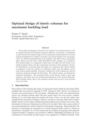
Then, the optimal distribution of the material a is determined from the relation@H2p m 0 1 @aa3pm ():2(a)(45)The corresponding costate equations and natural boundary conditions arep m @Hp 2;@map pm (1 2) 0;@H @pmaa;p (0) 0:We note that from Eqs. (45) and (47) it followsp() (0) pm (0);a (0) (46)(47)(48)as a new result that generalizes the one given by Eq. (15). According to Eq. (48) theshape of the optimal column at its end depends on the load and material. In other wordsthe optimal shape becomes sensitive of the load and it seems it will t for real columns.In order to get the optimal shape for several values of and we calculate Eulerbuckling load rst cg and then we solve two point boundary value problem (44),(46) and (47) with a obtained as a solution of Eq. (45). At each step of integratingprocedure Eq. (45) is solved numerically by bisection method. All numerical integrationsfor shooting method were based on Bulirsch-Stoer integration procedure [23]. In Table1. we present minimum half volume vmin , the minimal and the maximal area of thecolumn cross section, that is, amin a (0) and amax a (1 2) : For comparison, in Table1 Clausen solution, that corresponds to zero values of and ; and the critical value2 9:869, here obtained by numerical solution of the column problem. as a specialc case is also presented.Table 1.vmin amax a (1 2) amin a (0)0.00.09.869 0.4331.154700.0003 0.0001 9.868 0.4331.15480.01870.003 0.001 9.850 0.4341.15520.05980.030.01 9.670 0.4401.15840.19590.30.17.676 0.4761.14710.6693The optimal shapes of the column that correspond to several values of column parameters obtained by numerical integration of two point boundary value problem (44), (46)and (47), with a obtained as a solution of Eq. (45), are presentedp in Figure 5. As before,in Figure 5, we present optimal curve obtained as Ropt (t) aopt (t); which accordingto Pearson formulation of the Lagrange problem, gives the column of greatest e ciency.
Figure 5. Optimal shapes that generalize Clausen’s solution.We note that nite values of shear and extensional rigidity did change Clausen’s solution as expected. We conclude by noting that, along the lines of Keller [3] or Atanackovic[35], the results presented here could be generalized by introducing imperfections in theshape and loading and by allowing di erent boundary conditions. An interesting type ofboundary conditions, applicable to optimal design of water tower is presented in Spasicand Glavardanov [36].3Optimal shape of the column against spatial bucklingIn this section we wish to consider the buckling of a column subjected to a twisting coupleand compressive axial load. The ends of the column are assumed to be attached to thesupports by ideal spherical hinges and are free to rotate in any directions. As before onehinge is xed whereas the other one is free to move along the axis z: We as
solutions, that follow from two possible generalizations of the classical Bernoulli-Euler bending theory, lead to the optimum column with non-zero cross sectional area at its ends. 1 Introduction The problem of determining that shape of compressed column which has the largest Euler buckling load was posed by Lagrange in 1773.