WIXLIB

EDBT 2022, 29th March-1st April, 2022, Edinburgh, UKM. Hershcovitch, A. Khyzha, D. Waddington, and A. MorrisonElastic indexes This paper proposes to rein in index memoryoverhead by making it elastic. We propose an elastic indexdesign framework, which transforms an index with internal-keystorage into an elastic version.Under normal conditions, the elastic index is identical to thestandard index, leveraging the extra space provided by limitedmemory over-provisioning for its key storage and thereby offering optimal query performance. However, when a large amountof data is ingested, the elastic index temporarily shrinks itselfuntil memory pressure subsides. To dynamically shrink itself,the elastic index switches a portion of the nodes to a compactrepresentation with indirect key storage. Once memory pressure subsides, the converted nodes gradually revert back to theiroriginal form, storing keys internally.The elastic index framework can be applied to any index withinternal key storage, such as a B -tree, skip list, or Bw-Tree. Thedesign is parameterized by (1) the elasticity algorithm, whichadjusts the index’s space utilization by deciding when and whichnodes should start/stop using indirect key storage; and (2) thecompact node representation, which determines the space vs.query efficiency tradeoff.To demonstrate the design framework, we devise an elasticB -tree. For the elasticity algorithm, we propose a method thatpiggybacks on node splits and merges as the point in time toconvert regular nodes to/from blind tries [13]. For the compactnode representation, we propose a novel blind trie representation.Our blind trie obtains space efficiency comparable to the mostcompact blind trie in the literature [12] but with query complexitycomparable to that of faster, but less compact, representations [4,13].We evaluate the elastic B -tree using uniform and YCSB workloads, as well as by integrating it into the MCAS in-memorydata store. We find that an elastic version of the STX B -tree [2]can store 2 /5 the number of 8-byte/30-byte keys with only a25% throughput degradation. To evaluate the space/performancetrade-off of the elastic B -tree in a full system, we evaluate theMCAS [29] in-memory data store on a workload modeling ingestion and querying of cloud log data. Depending on the elasticityparameters, the elastic B -tree consumes from 0.76 to 0.3 the space of the default B -tree index, with only 0.5% to 2.6%degradation in query throughput.Giving up internal-key storage? Internal-key storage is fundamental to the performance of index operations. In principle,comparison-based in-memory indexes such as B -trees couldavoid internal-key storage by using indirection, i.e., by storingpointers to keys’ tuples and loading a key from the database whenan index operation needs to read it for a comparison. However,such a design would eliminate the spatial locality of having keysco-located in index nodes, which means that any key access bythe index would incur CPU cache misses, severely slowing downindex operations.A similar problem exists with index designs based on Patriciatries [21], such as HOT [3]. These indexes do not rely on keycomparisons and so are able to store keys indirectly withoutcompromising index point query performance. Unfortunately,large scans—which are common in analytics workloads [15, 24]—slow down significantly if each scanned key has to be loadedfrom the database (see § 6). Included-column queries [20]—i.e.,whose result is computed solely from the values composing thekey and the included columns—are similarly slowed down.Using prior index compression schemes? The elastic index approach provides better trade-offs than prior index nodecompress schemes. The overhead of general-purpose compression [22]—i.e., decompressing and re-compressing each accessedindex node—is significantly higher than the indirect key accessesperformed on nodes compacted by an elastic index. While prefix compression [14, 23]—which compresses a B -tree leaf bystoring redundant prefixes only once—is cheap, its compressionratio depends on the key distribution and it might even increasespace usage if keys do not share common prefixes. In contrast,switching a node to a compact representation always saves space.Using hybrid indexes? Hybrid indexes [33] improve indexspace efficiency using a two-stage architecture, in which recentlyadded data is held in a small dynamic index while a compact, readonly index holds the bulk of the index entries. A periodic mergeprocess migrates aged entries from the small dynamic index tothe compact index. Because the compact index does not supportindividual-key updates, the merge process must rebuild it entirely.In contrast, the elastic index design is fine-grained, convertingindividual nodes to/from a compact representation, and supportsupdates of the compact nodes. Moreover, the efficiency of thehybrid index approach is predicated on a skewness assumption—that updated index entries are those recently inserted. The elasticindex design does not require this assumption.Contributions We make the following contributions:(1) The elastic index design framework, which enables stretchinga fixed memory budget while gracefully degrading when largeamounts of data are consumed.(2) Applying the framework to construct an elastic B -tree.(3) A novel blind trie representation, which serves as the mainbuilding block of the elastic B -tree.(4) Empirically evaluating our algorithm against the state of theart indexes in the literature.23ELASTIC INDEX FRAMEWORKThe elastic index framework takes a baseline index whose nodesinternally store indexed keys (e.g., a B -tree or skip list) andtransforms it into an elastic index. Under memory pressure, anelastic index can trade off some query efficiency for better spaceefficiency by dynamically converting its data structure nodes intoa compact representation, which stores keys indirectly insteadof explicitly.Our framework targets the baseline index’s leaf nodes, whichare where index searches terminate, because these nodes occupymost of the space in the index. The observation underlying theelastic index transformation is that such leaves can be viewed as“mini indexes”—as they map from keys to database tuples—withtheir own abstract data type (ADT) interface. For example, theB -tree leaf ADT supports six familiar operations [6]: insert, remove, find, predecessor/successor, split, and merge. Therefore, acompact node representation that implements the leaf ADT canTHE CASE FOR ELASTIC INDEXESWe make the case for elastic indexes by explaining why existing approaches for addressing DBMS index size overheads aresuboptimal for our setting. We consider only ordered indexes—such as B -trees or tries—that support iteration, range selection,etc. in addition to point queries. The reason is that in-memoryDBMSs serve as data pipeline elements to support analytics, monitoring, and decisioning queries, which require multiple orderedsecondary indexes.313

Elastic Indexes: Dynamic Space vs. Query Efficiency TuningEDBT 2022, 29th March-1st April, 2022, Edinburgh, UKco-exist in the index with the standard leaf nodes, without anychanges to the baseline index algorithm. In turn, the co-existenceof regular and compact leaves allows devising an elasticity algorithm that responds to changing memory pressure by switchingleaves to/from their compact representation.The elastic index framework is parameterized by the following:The elasticity algorithm relies on a grow/shrink policy toselect which leaves to compact/decompact when the indexgrows/shrinks. In the following, we describe the algorithm witha policy that chooses leaves which experience B -tree overflow/underflow events due to insertions/removals. There is, however, a design space of possible policies. For example, the policycould pick infrequently accessed nodes for compaction, to minimize the impact on query speed. We leave exploration of differentpolicies to future work.The elasticity algorithm assumes that the compact leaf representation provides leaves of varying capacity, i.e., maximumnumber of keys that can be stored. The capacity of a leaf determines its size; the more compact the representation, the greatercapacity that can be offered by a (compact) leaf of size S. Theelasticity algorithm requires that a compact leaf with capacity of2n keys be smaller than a standard B -tree node with capacity ofn keys. (Blind trie representations, including ours, typically satisfy this property.) Other than these requirements, the elasticityalgorithm is agnostic to the compact representation. The compact node representation. The representation mustsupport the original index’s leaf operations. Designing a goodrepresentation requires carefully balancing compactness andthe efficiency of leaf operations. While the elastic index tradesoff some query efficiency for space efficiency, the goal is tominimize impact on query efficiency. The elasticity algorithm. This algorithm monitors indexspace consumption. In response to an increase in the database size, it begins converting leaves to the compact representation. When the database size reduces, it converts compactleaves back to the normal representation. The algorithm mustrespond to change in memory consumption as quickly as possible while minimizing interference on index operation undernormal conditions. The main challenge in designing an elasticity algorithm is how to pick the leaves that will be compacted.Shrinking When index size grows close to the size bound, theelasticity algorithm enters a shrinking state. In the shrinkingstate, the algorithm’s goal is to absorb insertions while (1) reducing the memory consumed by leaf nodes and (2) not increasingmemory consumption by inner nodes. We achieve this by modifying the way in which a leaf overflow is handled. Normally,an insertion about to overflow a leaf will split the leaf into twonew leaves, which requires further insertions of separators in theleaf’s ancestor inner nodes. Our algorithm piggybacks on thisoperation, which is already costly and infrequent1 and replacesthe leaf through a compacting operation.In the shrinking state, upon an insertion attempt into a fulln-key standard leaf, the elastic B -tree replaces the leaf with acompact node with a capacity of 2n keys (instead of splitting).The compact node is initialized to contain the original leaf’s nkeys and tuple identifiers. The insertion is then performed intothe new compact leaf. As a result, we save space in two ways:the new compact leaf is smaller than the original leaf, and noinsertions—possibly causing more splits—need to be performedat the upper layers of the tree.Subsequent insertions into the compact node might drive itsoccupancy to the capacity, creating an overflow. Typically, wehandle the overflow as before, by replacing the overflowing compact leaf with a compact leaf with double the capacity. Whilethis increases the size of the leaf, it still saves changes in theinner nodes. However, as a compact leaf grows larger, querieson it become slower (§ 5). Therefore, the elastic B -tree capsthe maximum capacity that a compact leaf may reach due tooverflow handling. An overflow of a compact leaf with maximumcapacity results in a split of that leaf. In practice, we have foundthat starting from a capacity of 16 keys and capping it at 128 keysworks well (§ 6).The elasticity algorithm maintains an invariant for compactleaves that is similar to the invariant of B -tree leaves, namely,that a compact leaf with a capacity of 2k keys must contain at leastk 1 keys. A remove operation that would bring a compact leafbeyond its lower threshold—cause an underflow—either replacesthe compact leaf with a compact leaf with capacity k, if k isgreater than the capacity of a B -tree leaf, or simply replaces thecompact leaf with a standard B -tree leaf.Choosing these “parameters” creates a large design space.Here, we initiate exploration of the design space by presenting an elastic B -tree based on two main ideas: (1) basing thecompact representation on a novel blind trie [13] representation(§ 5) and (2) having the elasticity algorithm piggyback on B -treesplit/merge operations as the point to efficiently convert leavesto/from the compact representation (§ 4).4B -TREE ELASTICITY ALGORITHMOur B -tree’s elasticity algorithm operates by striving to keepthe size of the index constant once it reaches a certain threshold, and leveraging the conversion of leaves to their compactrepresentation to index more keys with a fixed memory budget.The idea is to detect a window of time in which significantlymore data than usual is ingested. In such a case, the index istemporarily shrunk to make room for the extra data.The algorithm is configured with a soft size bound that indicates the maximum size the index should be allowed to growto. The algorithm attempts to keep index size below this bound.When the index size grows close to the bound (e.g., reaches 90%of it), the algorithm enters a shrinking state and starts converting leaves to the compact representation, which can index moreitems without increasing the index’s overall memory consumption. When the index size decreases because the data set sizedecreases, the algorithm enters an expansion state and starts converting leaves back to the standard representation. To preventscenarios of oscillation between shrinking and expansion, thealgorithm uses different thresholds for triggering shrinking andexpansion. That is, the algorithm switches from shrinking toexpansion only when the index size decreases far enough fromthe size bound.The elasticity algorithm works by compacting the index incrementally as the dataset grows, resulting in compact and standard nodes co-existing in the same tree. This approach minimizes overhead on index operations, in contrast to existing approaches that compact the entire index in bulk [33], which cantake significant time. Our incremental approach also results ina smoother space/efficiency trade-off, as only queries touchingcompact nodes become slower.1 The314amortized cost of a split in a B -tree is O (1).

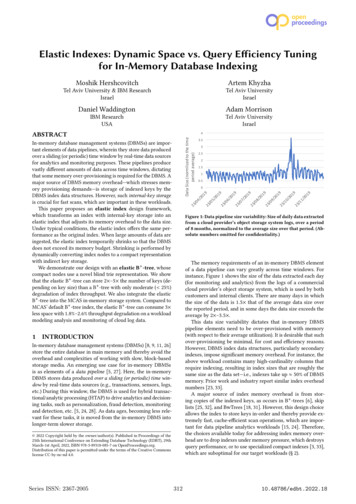
EDBT 2022, 29th March-1st April, 2022, Edinburgh, UKM. Hershcovitch, A. Khyzha, D. Waddington, and A. MorrisonExpansion When index size decreases far enough from thesize bound, the elasticity algorithm enters an expansion state, inwhich it strives to regain query performance by switching compact leaves back to the faster standard leaf representation. Theexpansion process undoes the steps taken during the shrinkingstate. Expansion occurs in two ways, as follows.One part of the expansion process occurs naturally as a consequence of removes, which are frequent operations once thedataset size starts decreasing. As explained above, a remove thatunderflows a compact leaf replaces it with a smaller compact leaf,and eventually with a standard leaf.The second aspect of the expansion process is aimed at casesin which a compact leaf becomes popular but does not experience removals. Such a leaf could potentially offer queries lowerperformance indefinitely. To avoid this problem, the elasticityalgorithm modifies the behavior of searches as follows. In the expansion state, a search that ends at a compact leaf with a capacityof 2k keys may randomly decide to split the leaf into leaves ofcapacity k. If k is equal to the B -tree leaf capacity, we split intostandard leaves; otherwise, we split into compact leaves.5and p is the tuple identifier size. The constant factor behind theO(·) notation is determined by the blind trie’s representation. Forexample, we would like to avoid storing pointers to children ineach node.Blind trie representations of B-tree nodes Work onexternal-memory B-trees has explored replacing the B-tree’s standard node structure of a sorted key sequence with some blindtrie representation. Let n be the capacity of the B-tree node. Theblind trie representations leverage the fact that n is small (say,n 256).The String B-Tree [13] uses a straightforward representation,in which each trie node contains two pointers to its children.Suppose that the index of a discriminating bit can be representedwith 1 byte (i.e., the key size k 32 bytes) and that a pointer to atrie node requires 1 byte (recall n 256). Then this representationrequires 3 B (bytes) per key (ignoring tuple identifiers). Bumbulisand Bowman [4] proposed a more compact representation thatwe call SubTrie. The SubTrie stores the nodes in an array sortedin pre-order (depth-first) traversal order of the trie. In this order,a node’s left child (if it exists) is simply the adjacent node in thearray. To facilitate finding right children and determining if aleft child exists, the SubTrie also maintains an array in which thei-th entry stores the size of the i-th node’s left sub-tree (inclusiveof the node). The SubTrie thus requires 2 B per key, under thesame assumptions on key size and number of keys. The densestrepresentation, which we call SeqTrie, is due to Ferguson [12]. Itrequires only 1 B per key, but its search complexity is linear inthe number of indexed keys (see § 5.2 for details).COMPACT NODE REPRESENTATIONHere, we describe SeqTree, our blind trie representation, whichserves as the compact representation of our elastic B -tree nodes.In § 5.4 we describe an optimization to reduce the space occupiedby the tuple identifiers stored in the node.Recall that we target a database indexing setting. In this setting,the index is indexing rows of a DBMS table, so the “values” storedin the index are tuple identifiers (pointers to rows of the table).In particular, the key can be extracted from the row it indexes(e.g., the key is the value of a specific column). This property isexploited by indexes such as HOT [3] to avoid storing explicitcopies of the keys. Instead, the search path in these indexes isdetermined by the searched key’s bits and they load a stored keyfrom the database table at the last step of the search, to checkwhether it matches the searched key.5.15.2The SeqTree representationWe present SeqTree, a blind trie representation whose space efficiency is comparable to the SeqTrie but with improved searchtime. The SeqTrie obtains optimal space efficiency by storingonly an array of size n 1 whose entries are the discriminating bits—without any auxiliary information. However, a SeqTriesearch must sequentially scan this entire array. Our observationin SeqTree is that this search can be sped up considerably bymaintaining a small auxiliary tree that helps a search quicklyidentify a small range in the array in which its result is found,and thereby reduces the length of the sequential scan it must perform. The storage cost of the auxiliary tree is negligible, becausethe blind trie is only meant to replace a B -tree leaf, and so itstores a small number of keys. As a result, the SeqTree’s spaceefficiency in practice is comparable to the SeqTrie’s but its searchperformance is comparable to the SubTrie.Next, we explain the SeqTrie representation and how it issearched. We then explain how the SeqTree algorithm is obtained by adding a small auxiliary tree to the SeqTrie, which isused to locate the range within a target key must reside withoutperforming a full sequential scan of the array.Background: Blind triesA trie is a search tree in which the position of a node in the treedefines the key associated with it: the root is associated with theempty string, and all descendants of the node associated withkey k share the common prefix k. A compressed trie is a pathcompressed representation of a trie in which the edges in everynon-branching path are merged into a single edge. Figure 2bdepicts a compressed trie indexing the keys in Figure 2a. Becausethe edges on a search path contain all key bits, a compressed triestores keys directly, just without duplicating common prefixes.A blind trie (also known as Patricia trie [21]) is a compressedtrie that does not label the edges but instead records in eachnode the position of the bit in which the node’s children differ.The blind trie does not explicitly store all key bits, and so ismore compact than a compressed trie. Figure 2c shows a blindtrie for the same set of keys. A blind trie search proceeds byexamining the discriminating bit indicated in the current nodeand continuing to the appropriate child. However, to complete asearch, the algorithm must look up the indexed tuple (pointed toby the leaf) to confirm that the indexed key matches the searchedkey.A blind trie requires only one node to be inserted for everyunique key stored. Its memory consumption is thus O(np (n 1) log k) bits, where n is the number of keys, k is the size of a key,SeqTrie The SeqTrie maintains an array in which entry i contains the first bit discriminating between the i-th and (i 1)-thkeys, where the keys are sorted in lexicographic order and bitsare numbered from zero, starting from the most significant bit(see the rectangles in Figure 2a). The SeqTrie representation ofour example key set is shown in Figure 3a as the array namedBlindiBits. We use this name as the array contains the discriminating bits of the blind index (Blindi). The SeqTrie also stores anarray with the values associated with the stored keys, denotedV 0, . . . , V 6 (as in Figure 2c).315

Elastic Indexes: Dynamic Space vs. Query Efficiency TuningmsbEDBT 2022, 29th March-1st April, 2022, Edinburgh, UKLsb#dec 01 234567 8165d 01 010010 1166d 01 010011 0170d 01 010101 0171d 01 010101 1214d 01 101011 0233d 01 110100 1235d 01 110101 2V0(a) Indexed keys and their binary V1V2V0V6V5RowIdKey166d(b) Compact 171d11RowIdKey233dRowIdKey235dV6V5V3(c) Blind trie.Figure 2: Different tries indexing a 7-row table whose rows are indexes by keys shown in (a). Rectangles mark the first bit in which twoconsecutive keys differ. The notation V x refers to the value associated with the x -th key, e.g., a tuple l1Level2587V457V4V5V3V2V1V0V6(a) SeqTree arrays. BlindiTree is the physical layout of the tree shown in (b).BlindiBits is the trie’s SeqTrie representation. Numbers above array entriesindicate their index.V5V6(b) SeqTree logical representation. The boxed number next to a node showsits index in the BlindiBits array.Figure 3: SeqTree representation for the key set of Figure 2a with tree of height vel1BlindiTree4Level2278V57V5V6(a) SeqTree arraysV07V4V1V2V6V3(b) Insert logic representationFigure 4: SeqTree representation for the key set of Figure 2a, after insertion of the mapping 186 7 Vins e r t .SeqTrie search The search has predecessor semantics, i.e., itreturns the position of the searched key or, if the searched key isnot indexed, the position of the largest key smaller than it. (Thisenables insertions and range scans to use the search procedureto locate the position in which the key should be inserted or thescan should start, respectively.) Let SKey denote the searchedkey. The search proceeds under the assumption that SKey is oneof the indexed keys. It scans the array sequentially, attemptingto find SKey’s position. Initially, we assume SKey is the first key(indexed 0). Suppose we assume SKey is the j-th key and we scanentry i. Let bi BlindiBits[i]. Then bit bi is 0 in the i-th key but 1in the (i 1)-th key. Thus, if SKey[bi ] 1, it cannot be that SKeyis the i-th key (or any smaller key). We call this case a hit, andwe now assume tht SKey’s position is i 1. If SKey[bi ] 0, thenSKey cannot be the (i 1)-th key, but our assumption that SKeyis the j-th key may still be true. We call this case a miss. Followinga miss, we need not check any discriminating bit b bi , becausefor any such entry, the relevant key has bit bi set and thereforecannot be SKey. We thus keep scanning the array but ignore anysuch bit.At the end of the sequential scan, the “assumed” position j willbe SKey’s position if SKey is one of the indexed keys. We verifythis by loading the j-th key from the database and comparingit to SKey. If they do not match, then we now know the bit bddiscriminating SKey and the j-th key, as well as whether SKeyis greater or smaller than the j-th key. Suppose SKey is greaterthan the j-th key. To find SKey’s successor, we scan the arrayto the right of the j-th entry, looking for an index i such thatbi BlindiBits[i] bd . This means that the (i 1) key has bitbi set and is therefore larger than SKey, but the i

storage into an elastic version. Under normal conditions, the elastic index is identical to the standard index, leveraging the extra space provided by limited memory over-provisioning for its key storage and thereby o er-ing optimal query performance. However, when a large amount of data is ingested, the elastic index temporarily shrinks itself