WIXLIB

NEWTON’S METHOD AND FRACTALSAARON BURTONAbstract. In this paper Newton’s method is derived, the general speed ofconvergence of the method is shown to be quadratic, the basins of attractionof Newton’s method are described, and finally the method is generalized tothe complex plane.1. Solving the equation f (x) 0Given a function f , finding the solutions of the equation f (x) 0 is one of theoldest mathematical problems. General methods to find the roots of f (x) 0 whenf (x) is a polynomial of degree one or two have been known since 2000 B.C. [3]. Forexample, to solve for the roots of a quadratic function ax2 bx c 0 we mayutilize the quadratic formula:x b b2 4ac.2aMethods to solve polynomials of degree three and four were discovered in the16th century by the mathematicians dal Ferro, Tartaglia, Cardano, and Ferrai [3].Finally, in 1826 it was discovered from work done by Abel, that there is no generalmethod to solve polynomials of degree five or greater [3].Since it is not possible to solve all equations of the form f (x) 0 exactly, anefficient method of approximating solutions is useful. The algorithm discussed inthis paper was discovered by Sir Issac Newton, who formulated the result in 1669.Later improved by Joseph Raphson in 1690, the algorithm is presently known asthe Newton-Raphson method, or more commonly Newton’s method [3].Newton’s method involves choosing an initial guess x0 , and then, through aniterative process, finding a sequence of numbers x0 , x1 , x2 , x3 , · · · 1 that convergeto a solution. Some functions may have several roots. Later we see that the rootwhich Newton’s method converges to depends on the initial guess x0 . The behaviorof Newton’s method, or the pattern of which initial guesses lead to which zeros,can be interesting even for polynomials. When generalized to the complex plane,Newton’s method leads to beautiful pictures.In this paper, we derive Newton’s method, analyze the method’s speed of convergence, and explore the basins of attraction2. Finally, we extend Newton’s methodto the complex plane, and through the aid of computer programming view thecomplex basins of attraction for several polynomials.1

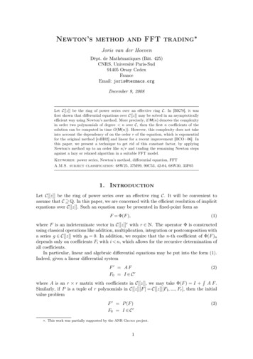
2AARON BURTONFigure 1. The geometry of Newton’s method2. Deriving Newton’s methodAs stated in Section 1, Newton’s method involves choosing an initial approximation x0 , and then, through an iterative process, finding a sequence of numbersx0 , x1 , x2 , x3 , · · · that converges to a solution. Recall our goal is to approximatethe root of a function f (x), thus once we chose our x0 we hope to find a point x1(related to x0 in some way) that is a better approximation for the root of the function f (x). Given a single point x0 there are many ways in which we could proceedto find the point x1 . In this paper we will use the tangent line at x0 . The tangentline provides the best linear approximation to the function f (x) at the point x0 ,thus we are implicitly assuming that the tangent line will intersect the x-axis nearthe desired root. This assumption seems to be valid based on Figure 1. In Section2 we will discuss how this assumption breaks down under certain circumstances.Now, suppose f (x) is a differentiable function on an interval [a, b] for which wewish to approximate the root. We begin by making a guess or estimate of theroot’s location, that is specifying an initial point (x0 , 0). To determine our nextestimate (x1 , 0), we draw the tangent line through (x0 , f (x0 )). The point at whichthe tangent line intersects the x axis is (x1 , 0). Using our initial guess x0 , the valueof the function f (x0 ) and the slope of the tangent line f 0 (x0 ) we can then find theequation of the tangent line at (x0 , f (x0 )) using the point-slope formula:y f (x0 ) f 0 (x0 )(x x0 ).To solve for the x intercept we set y 0 and rearrange terms to get f (x0 ) f 0 (x0 )(x x0 )1Often called the orbit of x .02Formally defined in Section 6, a Basin of Attraction is the set of points which converge to aparticular root.

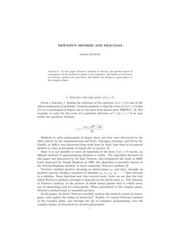
NEWTON’S METHOD AND FRACTALSx x0 f (x0 )f 0 (x0 )x x0 f (x0 ).f 0 (x0 )3and finally0)The x intercept is our new guess, or estimate, x1 . Thus we have, x1 x0 ff0(x(x0 ) .To find x2 , we begin the whole process over again. However, this time we beginwith the point (x1 , 0) and solve for the point (x2 , 0). Repeating this algorithmgenerates a sequence of x values x0 , x1 , x2 , · · · by the rulexn 1 xn f (xn ), f 0 (xn ) 6 0f 0 (xn )we define as the Newton iteration function N (x). Formally, given a differentiablefunction f , the Newton function for f is:(1)N (x) x f (x).f 0 (x)Thenx1 N (x0 )x2 N (x1 ) N (N (x0 )) N 2 (x0 )and, in general,xn N n (x0 ),where the notation N n means N applied n times.3. Where Newton’s method failsOne natural question that arises is whether Newton’s method will always converge to a root.3.1. Initial guess is a critical point of f (x). Recall from equation (1) that thedefinition of the Newton iteration function isN (x) x f (x).f 0 (x)From this definition we see that N (x) will not exist if f 0 (x) 0. If we chose aninitial point where f 0 (x) 0, then Newton’s method will fail to converge to a root.Similarly if f 0 (xn ) 0 for some iteration xn , then Newton’s method will also fail toconverge to a root. The former case is illustrated for f (x) x3 1 in Figure 2. Ifwe happen to choose our initial guess as x 0, Newton’s method fails to convergesince the tangent line at x 0 never intersects the x axis.3.2. No root to find. Another way in which Newton’s method will fail to convergeto the root of a function is if there is no root. Consider the graph of f (x) x2 1in Figure 3. The function f (x) x2 1 never crosses the x axis, and thus there isno possible solution. If we choose an initial guess, it can be proved that Newton’smethod will chaotically move around the x axis.3

4AARON BURTONFigure 2. f (x) x3 1. The initial guess coincides with a critical point.3.3. Periodic cycle. A third way in which Newton’s method will fail to convergeis if the initial guess or an iteration coincides with a cycle. For example, considerf (x) x3 2x 2 and the initial guess of x0 1 as shown in Figure 4. Withx0 1 we see that13 2(1) 2x1 N (x0 ) 1 1 1 0,3(1)2 2and then03 2(0) 2x2 N (x1 ) 0 0 ( 1) 1.3(0)2 2This example is of a cycle with period two, but cycles of other orders may exist aswell.4Often the problems just described can be avoided by choosing our initial pointwisely and by looking at the derivatives of the function to be approximated. Usuallyit is helpful to graph the function f (x) if possible before using Newton’s method.3For further details, refer to Devaney Chapter 13.2 example four.4See Devaney Chapter 3.3 for an in depth explanation of cycles.

NEWTON’S METHOD AND FRACTALSFigure 3. f (x) x2 1. Nonexistent root.Figure 4. f (x) x3 2x 2. A cycle of period 2.5

6AARON BURTON4. ConvergenceA natural extension of Section 3 is the question of convergence. When exactlycan we be sure Newton’s method will converge to a root? First a few backgrounddefinitions and a lemma.Definition 4.1. A root r of the equation f (x) 0 has multiplicity k if f (r) 0,f 0 (r) 0,· · · , f [k 1] (r) 0 but f [k] (r) 6 0. Here f [k] (r) is the k th derivative of f .For example, 0 is a root of multiplicity 2 for f (x) x2 x3 and of multiplicity1 for f (x) x x3 .Definition 4.2. A point x0 is a fixed point of a function f (x) if and only iff (x0 ) x0 . Moreover, the point x0 is called an attracting fixed point if f 0 (x0 ) 1.For our purposes it suffices for the reader to note that if a root is an attractingfixed point of the function N (x), then Newton’s method will converge to that point.For more information about fixed and attracting fixed points refer Appendix A.Lemma 4.1. If r is a root of multiplicity k for a function f (x), then f (x) may bewritten in the formf (x) (x r)k G(x), where G(r) 6 0Proof. Consider the Taylor expansion of a function f (x) centered about the root r.f 000 (r)f 00 (r)(x r)2 (x r)3 · · ·2!3!Now suppose that the root r has a multiplicity k. From the definition of multiplicitywe have,f (x) f (r) f 0 (r)(x r) 0f {k} (r)(x r)2 · · · (x r)k HOT2!k!f {k} (r) (x r)k HOTk!where HOT stands for higher order terms. From each higher order term we mayfactor out (x r)k , so we havef (x) 0 0(x r) f (x) (x r)k G(x){k}where G(x) f k!(r) HOT and G(x) is a function that has no root at r, that isG(r) 6 0. If f is a polynomial, then the multiplicity of any root is always finite. 4.1. Newton’s Fixed Point Theorem. Now we are ready to prove Newton’smethod does in fact converge to the roots of a given f (x).Newton’s Fixed Point Theorem 4.2. Suppose f is a function and N is itsassociated Newton Iteration function. Then r is a root of f of multiplicity k 0 ifand only if r is a fixed point of N . Moreover, such a fixed point is always attracting.Proof. Suppose that f (r) 0 but f 0 (r) 6 0, that is, the root r has multiplicity 1.5Then from the definition N (x) x ff0(x)(x) , we have N (r) r. Thus, r is a fixedpoint of N . Conversely, if N (r) r we must also have f (r) 0.5Commonly known as a simple root.

NEWTON’S METHOD AND FRACTALS7To see that r is an attracting fixed point, we use the quotient rule to computef (x)f 00 (x)(2)N 0 (x) .(f 0 (x))2Again assuming f (r) 0 and f 0 (r) 6 0, we see that N 0 (r) 0. Since N 0 (r) 1,r is an attracting fixed point by definition. This proves the theorem subject toassumption that f 0 (r) 6 0.If f 0 (r) 0, then suppose that the root has multiplicity k 1 so that the(k 1)th derivative of f vanishes at r but the kth does not. Thus we may writef (x) (x r)k G(x)where G is a function that satisfies G(r) 6 0.6 Then we havef 0 (x) k(x r)k 1 G(x) (x r)k G0 (x)f 00 (x) k(k 1)(x r)k 2 G(x) 2k(x r)k 1 G0 (x) (x r)k G00 (x).Therefore, after some cancellation, we have(x r)G(x).N (x) x kG(x) (x r)G0 (x)Hence N (r) r, which shows that the roots of f correspond to fixed points of Nwhen r is a root of multiplicity k 1. Finally we computeN 0 (x) k(k 1)G(x)2 2k(x r)G(x)G0 (x) (x r)2 G(x)G00 (x)k 2 G(x)2 2k(x r)G(x)G0 (x) (x r)2 G0 (x)2(note (x r)2k 2 has been factored out of both the numerator and denominator).Now G(r) 6 0, sok 1 1.kThus, r is an attracting fixed point for N .N 0 (r) To reiterate, Newton’s Fixed Point Theorem tells us that the fixed points ofthe function N (x) are the roots of f (x). Furthermore, because the roots of f (x)are attracting fixed points for N (x), as we iterate N (x) the resulting sequence ofpoints, x0 , x1 N (x0 ), x2 N (x1 ), · · · , will converge to the root of f (x).5. An example of Newton’s methodAs an example of Newton’s method, we approximate the solution tof (x) x3 x 1 0.By examining Figure 5 it is clear that there is a exactly one root between 1 and 2.The Newton function for f (x) is:x3 x 12x3 1 .3x2 13x2 1Starting with the initial guess x0 1, the results of the iteration of the Newtonfunction are:N (x) x 6In the case of f 0 (r) 0, r is not in the domain of the corresponding function N (x); at r thereexists a removeable discontinuity. When we rewrite f using Lemma 4.1 we have removed thediscontinuity at r. This subtle difference between the two functions f (x) is of little consequencebut is mentioned here for the sake of completeness.