Transcription
Available online at www.sciencedirect.comScienceDirectProcedia Engineering 101 (2015) 235 – 2423rd International Conference on Material and Component Performanceunder Variable Amplitude Loading, VAL2015Fatigue life from sine-on-random excitationsFrédéric Kihma*, Andrew Halfpennya, Neil S. FergusonbaHBM-nCode Products Division, Technology Center, Brunel Way, Catcliffe, Rotherham, S60 5WG, UKbInstitute of Sound and Vibration Research, University of Southampton, Southampton SO17 1BJ, UKAbstractThis presentation concentrates on calculating the high cycle fatigue life from sine-on-random excitations. A spectraldomain approach offers advantages over the time domain approach when computation times are prohibitive.The proposed approach is to derive the statistical rainflow cycle histogram from a sine-on-random spectrum of stressdata and then to use the appropriate material fatigue curve to obtain the estimated life.A case study illustrates the application of the method on a component attached to a helicopter. Comparisons withtraditional time-domain approaches are presented and show excellent agreement. 2015PublishedThe Authors.PublishedbyisElsevierLtd. article under the CC BY-NC-ND license 2015by ElsevierLtd. Thisan open accessPeer-reviewunder responsibility of the Czech Society for nc-nd/4.0/).Peer-review under responsibility of the Czech Society for MechanicsKeywords: Random; Sine-On-Random; Fatigue; Damage; Rainflow Cycle Count1. IntroductionSine-on-random excitations are typically generated by rotating machinery. Sine-on-random excitations arespecified in international standards such as in MIL STD 810G [1] or in RTCA DO 160G [2].So far, the only way of estimating fatigue life from a sine-on-random excitation is to perform a transient analysisusing time domain realizations of the required PSD and harmonic tones as the excitation. Such an analysis can beaccelerated by using modal superposition but is still very demanding in terms of CPU time. It also raises the questionof how long the excitation signal should be to ensure convergence on fatigue life. The time domain approach istherefore impractical and this is the main reason why a spectral approach is relevant.* Corresponding author. Tel.: 33 130182020; fax: 33 130182019.E-mail address: Frederic.kihm@hbmncode.com1877-7058 2015 Published by Elsevier Ltd. This is an open access article under the CC BY-NC-ND nd/4.0/).Peer-review under responsibility of the Czech Society for Mechanicsdoi:10.1016/j.proeng.2015.02.033
236Frédéric Kihm et al. / Procedia Engineering 101 (2015) 235 – 242Fig. 1 shows example of rainflow cycle histograms obtained from various time domain realizations of a sine-onrandom spectrum. The first time series was 20 seconds long (red) and the later was 250 seconds long (blue). Theobtained rainflow histograms are scaled to 2000 seconds for comparison purposes. A statistical distribution (dashedblack) was obtained using the approach presented in this paper and superimposed with the time domain simulations.Fig. 1. Rainflow cycle histograms for various time domain realizations vs. spectral approach.Several observations can be made from Fig. 1x The longer the time domain simulation, the more chances there are to find cycles with high ranges.x Longer time domain simulations seem to produce rainflow histogram that converge towards the statisticalcycle distribution.x The tail of the statistical cycle distribution on the high-range end is well defined, allowing a more robust andaccurate fatigue life prediction from long term sine-on-random excitation.2. MethodologyEvaluating the fatigue damage due to a sine-on-random excitation requires a list of stress cycles together with afatigue curve for the material considered. The various steps involved to obtain the stress cycles are described below.The noise is assumed to be confined to a narrow band of frequencies, meaning that one mode is predominant. Thesine tone frequencies are supposed to be within the same frequency range as the noise. Finally, the sine tonesfrequencies are supposed to be incommensurable. In this case, the sine waves frequencies must be irrational relativeto each other. This means they can be considered independent and the relative phase has no importance.Generally, a sine-on-random signal can be represented as:Nx tr t b i .cos 2S f i t Mi(1)i 1with r(t) some random noise and bi, fi and φi the amplitude, frequency and phase of the N sine tones.Considering that a periodic signal can be decomposed into its Fourier coefficients, Equation (1) can be interpretedas a representation of deterministic periodic signal on random.The relative importance of the deterministic part in terms of power is indicated by the sine-to-random power ratio ଶ , given in Equation (2).a02V s2V r2N12V r2 bi2i 1with ߪ the RMS value of the noise and ߪ௦ the RMS value of the combined sine waves.(2)
237Frédéric Kihm et al. / Procedia Engineering 101 (2015) 235 – 2422.1. From sine-on-random acceleration spectrum to sine-on-random stress spectrumThe excitation is generally in the form of a PSD of acceleration with one or several superimposed sine tones, as inMIL STD 810G [1] or in RTCA DO 160G [2]. Assuming a linear structural response, one can derive the PSD of stressfrom the structure’s frequency response function H as per Equation (3). Similarly, the stress response to sinusoidalexcitation is determined from Equation (4).PSDstress fH f .PSDexcitation f .H * f(3)Sinestress fH f .Sineexcitation f(4)2.2. Transformation of the sine-on-random stress spectrum to the distribution of rainflow cyclesThe aim is now to find a statistically derived, rainflow-like distribution of cycles corresponding to the stress PSDand sine tones. S.O. RICE [3] derived the probability density function of peaks in the case where noise and harmonictones are within the same frequency range. The probability density function of peaks is given in Equation (5).ffp ss.³ x.e§ V 2 . x2 · r 2 ¹0NJ 0 x.s J0x.bi .dx(5)i 1where s is a random variable, representing the peak value, ܬ ܾ ǡ ǤClosed form solutions exist for the integral in Equation (5) when none or one harmonic tone is considered,numerical integration is required in the case of two or more tones are present.The rainflow cycle counting algorithm identifies stress cycles which ranges are calculated from the values of theirpeaks and valleys. The range of a rainflow cycle is defined as {peak – valley} of the cycle. The rainflow algorithmpairs peaks and valleys according to their value and position in the history of stress [4], for instance, the peak andvalley of a cycle are not necessarily consecutive.According to the assumptions made at the beginning of this section, the composite process made of narrowbandnoise and sine tones is narrowband too. This means that all peaks are positive and all valleys are negative. If the sinetones frequencies are not multiple of each other, each peak is associated with a valley of similar magnitude and thecycle’s range distribution can be determined from the peak distribution given in Equation (5). Therefore, the cycle’srange distribution is identical to the rainflow cycle distribution and is deduced from the peak distribution, as perEquation (6).f R SR1 § SR ·fp 2 2 ¹(6)When the noise corresponds to a multimodal stress response, i.e. more than one mode dominates, the noise isconsidered to be broadband. The bandwidth is characterized by the irregularity factor, a real scalar value calculatedfrom the spectral moments [3,5]. In the broadband case, due to the complex nature of the rainflow counting algorithm[4], the rainflow distribution for the cycles cannot be obtained from the peak distribution alone. However, consideringthat the largest cycle is always made of the highest peak and the lowest valley once residuals are closed [4], the useof equation (6) to calculate the range distribution is equivalent to considering that peaks and valleys are paired in themost severe way i.e. the highest peak goes with the lowest valley, the second highest peak goes with the second lowestvalley, etc. This narrowband approach is therefore expected to be conservative in the broadband case, as observed byRychlik [6] in the case of random processes.
238Frédéric Kihm et al. / Procedia Engineering 101 (2015) 235 – 242Other considerations like sine tones frequencies lying outside the noise frequency range or being multiples to eachother and influence of relative phases are currently under investigation.Considering random noise only, the total number of expected peaks per unit time Np can be derived by stating thata peak (i.e. a local maximum) is obtained from the number of zero crossings with a negative slope of the derivative ofthe process ሶ . Np is therefore calculated [3] by dividing ɐ ሶ ଶ with ɐ ሷ ଶ , referred to as the second and fourth spectralmoments of the PSD ܩ or the variances of the first and second derivatives of the random process respectively.In the sine-on-random case, the total number of expected peaks per unit time Np sor can be derived by extendingthe equation to obtain Np. The suggested extension consists in adding the spectral moments of the sine wave to thespectral moments of the noise. The averaged number of peaks per unit time calculated from the stress PSD and thesine waves characteristics is given in Equation (7).V r 2 1 2 1 f i 4bi 2NN p sor(7)V r 2 1 2 1 f i 2bi 2Nwhere ݂ and ܾ are the frequency and amplitude of the ith harmonic out of the N harmonics added to the noise. Thedistribution of fatigue cycles, comparable to a rainflow cycle histogram, can be calculated using equation (8):N SRf R SR .N p sor .T(8)where T is the exposure duration.2.3. Fatigue damageThe damage at a given stress range SR is obtained as the ratio of the cycles counted at this stress range level, to thenumber of cycles required to fail the component at this stress range level, which is given by the material curve likethe one illustrated in Fig. 2. The total damage is obtained by summing the damage from each individual level of stressrange using Miner’s rule [7].Fig. 2. Typical SN fatigue curve.The SN curve may be made of several segments. Each segment is represented as a straight line in log space asdescribed by the Basquin power-law relationship given in Equation (9).
239Frédéric Kihm et al. / Procedia Engineering 101 (2015) 235 – 242CN f .S R b(9)where ܵோ is the stress range in MPa, ܰ is the number of rainflow cycles to failure, C is the Basquin coefficient and bis the Basquin exponent. Fatigue damage is determined by Equation (10).D1Nff1N SR .S R b .dS RC ³0(10) Ǥ ͳ Ǥ ͳ Ȁ Ǥ 3. Industrial applicationThe present case study illustrates the use of the technique described in this paper to quantify vibration-inducedfatigue damage on a component attached to the fuselage of a helicopter. Helicopters are particularly challenging withregards to vibration.Standard vibration qualification tests are typically performed according to one of the commonly used militarydesign standards such as MIL-STD-810F [2], and RTCA DO-160E [3]. The endurance test commonly uses a sine-onrandom vibration profile which is representative of the actual aircraft loading profile. The main source of thesesinusoidal tones is attributable to harmonics of the main rotor.The component is flight safety-critical and the general vibration specification was considered inadequate in thiscase. A test tailoring exercise was therefore authorised to determine a more appropriate sine-on-random qualificationtest [8] using the ‘GlyphWorks Accelerated Testing’ package from HBM-nCode [9].3.1. The excitationThe vibration endurance test profile was compressed into 20 hours of high cycle fatigue in each axis. It is illustratedin Fig. 3. It is made of a random profile between 10 and 500 Hz with 2 gRMS and sine tones at rotors blade passingfrequencies and their harmonics (1nR,2nR,3nR) with amplitudes ranging between 0.1g to 2.0g. In most cases thevertical and lateral accelerations dominate the loading environment and the fore/aft axis is relatively benign. Only thevertical axis is discussed here.Fig. 3. Sine on random excitation spectrum used.3.2. Stress sine on random spectrum at critical locations
240Frédéric Kihm et al. / Procedia Engineering 101 (2015) 235 – 242Both a frequency response analysis and a transient analysis were performed. The frequency response analysis allowsfinding the spectral response in stress, whereas the transient analysis gives the time series response in stress.Results from two critical locations were retained for the present case study. Both results show very different sineto-random power ratios and irregularity factors, as reported in Table 1.Table 1. Characteristics of two responses.Location IDsine-to-randompower ratio ܽ ଶirregularity factorLocation 11.20.98Location 28.20.87The normal stress was calculated on multiple planes. This allows the computed damage due to the loads in X, Yand Z directions to be summed up in the same plane. The critical plane is the plane with the most predicted fatiguedamage. The responses shown in Fig. 4 and 5 are given for the same (critical) plane.Time domain realizations of 100 seconds, sampled at 1024 points per second were obtained from the excitationspectra in the various directions (see Fig. 3). The transient modal superposition analysis allows obtaining time historiesof stress responses at the various nodes. An example stress response is illustrated in Fig. 4.Fig. 4. Example stress response at Location 1Applying equations (3) and (4) to the transfer function obtained from the frequency response analysis, the sine-onrandom response in stress is obtained for Location 1 and 2 and illustrated in Fig. 5 (a) and Fig. 5 (b) respectively.Fig. 5. Sine on random stress response spectrum at (a) Location 1, (b) Location 23.3. Derived statistical rainflow distributions and damage– comparison with time domain
Frédéric Kihm et al. / Procedia Engineering 101 (2015) 235 – 242241The technique presented in this paper allows to evaluate the rainflow stress cycles distribution at every node of theFE model of a component subject to sine-on-random loading. The rainflow cycles distribution can also be obtainedfrom deterministic counting of the cycles in the time domain stress responses.Fig. 6 (a) and Fig. 6 (b) compare the rainflow cycles distributions obtained from deterministic counting of thecycles on the time domain stress responses (red) vs statistical approach (blue) for both critical locations 1 and 2.Fig. 6. Comparison between time domain (red) and statistical (blue) cycle distributions for (a) location 1 and (b) location 2From Table 1 and Fig. 5 (a) and 5 (b), location 1 can be associated to a unimodal narrowband response with sinetones which frequencies lie within the frequency band of the noise (except the lowest frequency one but it has thelowest amplitude). The sine tones have frequencies that are multiple to each other. The response at location 1 istherefore not respecting all the required assumptions to use the technique described in this paper. The response atlocation 2 is even worse in that respect as its irregularity factor is smaller, meaning it cannot be considered asnarrowband. However, in both cases the statistical approach is giving a good approximation of the deterministichistogram and it leads to a far better definition of the tail at the high ranges end, which is particularly important forfatigue analysis.Fatigue damage can be assessed from the rainflow cycle distributions obtained and an SN material curve. Table 2show the resulting damage calculated from an SN curve having a Basquin exponent of b 12.Table 2. Fatigue Damage.Location IDFatigue damage fromtime domainFatigue damage fromspectral domainLocation 116 E-323 E-3Location 226 E-336 E-3Again, the results from the spectral domain and time domain approaches are very similar, and so although some ofthe assumptions required to obtain the statistical rainflow histogram are not strictly respected. The fatigue damageobtained from the spectral approach is roughly 40% higher, mostly due to the best definition of the tail of the rainflowcycle distributions. The results from the spectral approach are more reliable as they implicitly take into account theprobability of high cycles appearing at long exposure durations.
242Frédéric Kihm et al. / Procedia Engineering 101 (2015) 235 – 2424. ConclusionsA spectral domain approach to fatigue analysis offers advantages over the time domain approach when limitedstress time history data are available or computation times are prohibitive. A very robust method of deriving fatigueestimates for sine-on-random vibration is presented.A case study illustrates the use of the method to assess the fatigue damage on a component attached to the fuselageof a helicopter. Comparisons with traditional time-domain approaches show excellent agreement. The results from thespectral approach are more reliable as they implicitly take into account the probability of high cycles appearing atlong exposure durations.Other applications of spectral fatigue analysis include finding out what the margins of a successful test are orchecking that a profile for random vibration test is not over accelerated. In this last case, the excessive loads introducelevels of stress above yield, which alters the load paths and change the failure mode.So far the existing approach for high-cycle fatigue damage assessment under random vibrations was limited toGaussian random loads. The new method extends it to multiple sine tones added to Gaussian random loads. This newmethod is particularly useful to take into account the vibration environment generated by rotating machinery.AcknowledgementsThe authors would like to acknowledge Paul Gardner for his help with the FEA analyses.References[1] "MIL-STD-810G: Test method standard for environmental engineering considerations and laboratory tests," United States Department ofDefense, 2008.[2] “RCA/DO-160 Revision G: Environmental Conditions and Test Procedures for Airborne Equipment”, RTCA, 2010[3].Rice, S.O., Mathematical analysis of random noise, Bell System Technical Journal, Vol. 23, pp. 282-332, 1944.[4] Downing S.D., Socie D.F. Simple rainflow counting algorithms. Int. J Fatigue pp 31-40. Jan, 1982.[5] Halfpenny, A., Rainflow Cycle Counting and Fatigue Analysis from PSD, Astelab, 2007[6] Rychlik, I., On the "narrow-band" approximation for expected fatigue damage. Probabilistic Engineering Mechanics, Vol. 8. pp. 1-4, 1993[7] Miner, M.A., Cumulative damage in fatigue," Trans. ASME, Journal of Applied Mechanics, Vol. 67, pp. A159-A164, 1945.[8] Halfpenny, A., Walton, T., C., Using the FDS to determine flight qualification of vibrating components on helicopters, Astelab, 2009[9] HBM-nCode. GlyphWorks Accelerated Testing User Manual. 2008.
MIL STD 810G [1] or in RTCA DO 160G [2]. Assuming a linear structural response, one can derive the PSD of stress from the structure's frequency response function H as per Equation (3). Similarly, the stress response to sinusoidal excitation is determined from Equation (4). .* PSD f H f PSD f H f stress excitation (3) Sine f H f Sine f