Transcription
(17E00103) MANAGERIAL ECONOMICSObjective of this course is to understand the relevance of economics in businessmanagement. This will enable the students to study functional areas of management suchas Marketing, Production and Costing from a broader perspective.1. Introduction to Managerial Economics: Definition, Nature and Scope, Relationshipwith other areas in Economics, Production Management, Marketing, Finance andPersonnel, Operations research - The role of managerial economist. Objectives of thefirm: Managerial theories of firm, Behavioural theories of firm, optimizationtechniques, New management tools of optimization.2. Theory of Demand: Demand Analysis – Law of Demand - Elasticity of demand, typesand significance of Elasticity of Demand. Demand estimation – Marketing researchapproaches to demand estimation. Need for forecasting, forecasting techniques.3. Production Analysis: Production function, Isoquants and Isocosts, Productionfunction with one/two variables, Cobb-Douglas Production Function, Returns toScale and Returns to Factors, Economies of scale- Cost concepts - cost-outputrelationship in the short run and long run, Average cost curves - Break Even Analysis.4. Market Structure and Pricing practices: Features and Types of different competitivesituations - Price-Output determination in Perfect competition, Monopoly,Monopolistic competition and Oligopoly. Pricing philosophy – Pricing methods inpractice: Price discrimination, product line pricing. Pricing strategies: skimmingpricing, penetration pricing, Loss Leader pricing. Pricing of multiple products.5. Inflation and Business Cycles:-Definition and meaning-characteristics of Inflationtypes of inflation - effects of inflation - Anti-Inflationary methods - Definition andcharacteristics of business cycles-phases of business cycle - steps to avoid businesscycleTextbooks: Managerial Economics -Analysis, Problems ,Cases ,Mehta,P.L., Sultan Chand &Sons. Managerial Economics, Gupta, TMHReferences Managerial Economics, D.N.Dwivedi,Eighth Edition,Vikas Publications Managerial Economics, Pearson Education, James L.Pappas and EngeneF.Brigham Managerial Economics, Suma Damodaran, Oxford. Macro Economics by MN Jhingan-Oxford Managerial Economics- Dr.DM.Mithani-Himalaya Publishers Managerial Economics-Dr.H.L Ahuja-S.Chand and Com pvt ltd, NewDelhi Managerial Economics by Dominick Salvatore, Ravikesh Srivastava- OxfordUniversity press. Managerial Economics by Hirschey- Cengage Learning1 Pa g eUNIT -3 PRODUCTION ANALYSISBALAJI INSTITUTE OF IT AND MANAGEMENT
UNIT-3PRODUCTION ANALYSIS1. PRODUCTION FUNCTION:1.1: PRODUCTION ANALYSIS:MEANING AND DEFINITION OF PRODUCTIONProduction analysis or theory of production deals with a relationship betweeninput factors and output the operational efficiency for optimum output andcost of production is not considered.ACCORDING TO JAMES BATES AND J.R. PARKINSON,” production is theorganized activity of transforming resources into finished products in the formof goods and services and the objective of production is to satisfy the demandof such transformed resources”.1.2: FACTORS OF PRODUCTION:Production requires the use of certain resources. Each particular resource maybe called a factor of production. Anything that contributes towards output is afactor of production. For the sake of convenience it is usual to group allproductive resources fewer than four heads land labor capital and organizationeach group being called a factor of production.PRODUCTION1. LAND: The term is used in different sense in economics. It does not mean soil or earth’s surface alone but refers to all freegift of nature which would include besides the land in commonparlance natural resources fertility of soil water air natural vegetationetc.2. LABOUR: The term labor means mental or physical exertion directed toproduce goods or services. In other words it refers to various types of human effort require theuse of physical exertion skill and intellect. Labor to have an economic significance must be one which is donewith the motive of some economic reward. Division of labor is animportant feature of modern industrial organization.2 Pa g eUNIT -3 PRODUCTION ANALYSISBALAJI INSTITUTE OF IT AND MANAGEMENT
3. CAPITAL: Capital may be defined as that part of wealth of an individual orcommunity which is used for further production of wealth. In fact capital is a stock concept which yields as produced means ofproduction.4. ENTREPRENEUR: It is the factor which mobilizes the other factors land, labor, andcapital; combines them in the right proportion then initiates theprocess of production and bears the risk involves in it. This factor is known as the entrepreneur. He has also been called theorganizer, the manager or the risk taker.1.3 PRODUCTION FUNTION: Production function states the relationship between inputs and outputi.e., the amount of output that can be produced with given quantities ofinputs under a given state of technical knowledge. The output takes the form of volume of goods or services and the inputsare different factors of production i.e., land, labor, capital andenterprise.Mathematically the production function is described as,Q f (X1, X2, X3 Xn)Where,Q Quantity produced during a given period of time(X1, X2, X3 .Xn) Quantities of various inputs used in production.Production function can also be defined in a different way. If shows theminimum quantities of various inputs that are required to yield a givenquantity of output.1.4: ASSUMPTIONS OF PRODUCTION FUNCTIONSThe production function has following assumptions,1. Perfect divisibility of both inputs and output2. Limited substitution on one factor for the other.3. The level of technology remains constant4. Inelastic supply of fixed factors in the short run5. It is related to specified period of time.1.5: SIGNIFICANCE OF PRODUCTION FUNCTIONS3 Pa g eUNIT -3 PRODUCTION ANALYSISBALAJI INSTITUTE OF IT AND MANAGEMENT
Production function analysis is of practical importance in managerial decisionmaking in business.Some of its managerial uses are given below,1. Production function analysis is of great of help in making shot perioddecisions by business executives in two ways.a. How to get optimum level of output from a given set of inputsb. How to get the given level of output from the minimum set of inputs.2. Production function analysis is of highly useful in making long perioddecisions by business executives If returns to scale are increasing it willbe worthwhile to increase production if returns to scale are diminishingit will be worthwhile to decrees production and if returns to scaleremain constant it would be indifferent to the producer whether toincrease or decrease production if demand is no constraint.3. Production function analysis is of great use to calculate the least costcombination of various factors in outs for a given level of output or themaximum output input combination for a given cost.4. Production function analysis is logical and also to common sense if theprice of one factor input falls while one for the second.5. Production function analysis is of great importance in making decisionon the utility of employing a variable input in the production process.1.6: LIMITATIONS OF PRODUCTION FUNCTIONSProduction function analysis has the following limitations.1. Production function analysis has restricted itself to the case of twoinputs and one output. Mathematically, there is no great difficulty inextending this analysis to multiple inputs and outputs.2. Production function analysis has assumed smooth and continues curveswhile in the real world, discontinuities in the production function mayappear.3. Production function analysis assumes that technology remains constant.But in reality it does not remain the same.4. Production function analysis is also applied under perfectly competitivemarket situations which are rare in the real world.5. Production function analysis assumes that units of labor arehomogeneous. In reality labor units are not identical but heterogeneousin characters.4 Pa g eUNIT -3 PRODUCTION ANALYSISBALAJI INSTITUTE OF IT AND MANAGEMENT
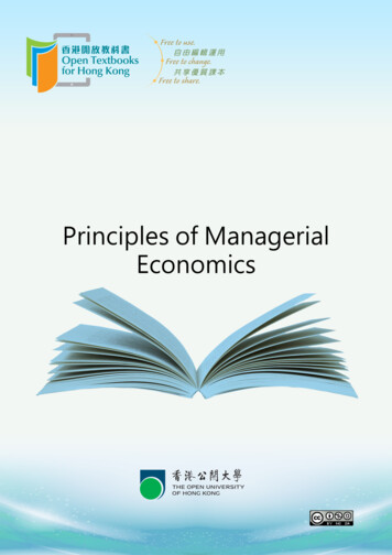
2. ISOQUANTS AND ISOCOSTS:2.1: MEANING AND DEFINITION OF ISOQUANTS Isoquant is also known as production function with two variable inputsor equal product curvesDEFINITION:According to FERGUSON, an isoquant is a curve showing all possiblecombinations of inputs physically capable of producing a given level of output. The combinations of all variable inputs which can yield the same outputwith various combinations are termed as isoquants. They are also known as iso-product or iso-product curve. For betterunderstanding of isoquants following schedule may be seen which givesvarious combinations of variable factors x and y for a given level ofoutput.factors x and y for a given level of output.Table 3.2: combination of two inputsFactor combinationFactor XFactor YA112B208C305D403E502Each of the factor combinations A, B, C, D and E represents the same levels ofproduction say 100 units. When we plot them we get a curve IQ as shown infigure 3.3Figure 3.3: equal productcurve or isoquant2.2: ASSUMPTIONS OF ISOQUANTSIsoquant analysis is normally based on the following assumptions1. It has been assumed that there are only two factors of input forgeometrical representation but in practice there are generally four orfive or even more variable used in production.5 Pa g eUNIT -3 PRODUCTION ANALYSISBALAJI INSTITUTE OF IT AND MANAGEMENT
2. It has been assumed that factors of production are divisible in smallunits and can be used in various proportions. In practice it not feasiblefor all factors.3. Technology constraints do not permit to change the input variables atany point of time.4. During production utmost care is taken to utilize the different factors inmost efficient way. This practice has not been followed in thisassumption.2.3: TYPES OF ISOQUANTSIsoquants assume different shapes depending upon the degree ofsubstitutability of inputs under consideration.1. LINEAR ISOQUANTS: In this case the inputs are replaceable in direct proportion. Forexample, a given amount of output say 200 units can be obtained byusing 2 units of labor or 1000 units of capital or 4 units of labor and500 units of capital. It can have various combinations. One more example say a particular village can be electrified by use ofcoal or solar power. The desired amount of electricity can begenerated by use of coal or by solar cell. The amount of powergenerated (say P1, P2, P3 P5) can be increased by increasing theconsumption of coal or increasing the installed capacity of solar cells.These two are substitute of each other. Hence in such cases theisoquants are straights lines as shown in,2. RIGHT-ANGLE ISOQUANTS: In such cases there cannot be any substitutability between theinputs. For example for plastering of a room requires 2 units of sandand 1 unit of cement there is no other way to substitute cement bysand (with no quantity compromise) and for increase in number of6 Pa g eUNIT -3 PRODUCTION ANALYSISBALAJI INSTITUTE OF IT AND MANAGEMENT
rooms of same size the quantity requirements of sand and cementwill increase in the same proportion. This is called Leontief or inputoutput isoquants as shown in figure 3.53. CONVEX ISOQUANT: In this case the substitution of inputs is not in totality. A particularassignment can be completed by employing minimum labor L1 intime T1. This assignment can still be completed in shorter periods T2and T3 by employing more labor i.e. L2 and L3. Increase in laborreduces the completion time from T1 to T2 and T3. To reach level of T3 required a significant increase in labor. Thus thesubstitutability of labor for time increases from L1 to L2 to L3.Further increase in labor has no benefit of time rather it is a waste.This is shown in figure 3.6.7 Pa g eUNIT -3 PRODUCTION ANALYSISBALAJI INSTITUTE OF IT AND MANAGEMENT
2.4: GENERAL PROPERTIES OF ISOQUANT CURVES:The properties of isoquants are describes below1. ISOQUANTS AE NEGATIVELY SLOPED: Generally isoquants sloedownwards in anticlockwise direction and follow a negative slope. This isdue to the fact that reduction of one input factor requirementsappropriate increase in other factor for maintaining the same level ofoutput.Figure3.7: isoquant having positively-sloped segments2. HIGHER ISOQUANT REPRESENTS A LARGER OUTPUT: the higherisoquant is one which can yield higher output by use of same amount ofone factor and higher amount of other factor or higher amount of boththe factors.Figure 3.8: two isoquants representing different outputlevels.3. TOW ISOQUANTS INTERSECT OR TOUCH EACH OTHER: since isoquantsrepresents different level of output and hence they do not intersect ortouch each other.8 Pa g eUNIT -3 PRODUCTION ANALYSISBALAJI INSTITUTE OF IT AND MANAGEMENT
4. ISOQUANTS ARE CONVEX TO THE ORIGIN: generally in productionprocesses substitutes can be arranged such as labor can be substitutedby capital and vice versa. However the marginal rate of substitution hasa decreasing tendency.Figure: convexity of an isoquant 2.5: ISOCOSTS:Iso-cost curve is the path traced by several combinations of L and Kwhere each of them requires the same amount of money for production.On differentiating the equation with respect to L we get dK/dL -w/r,that represents the slope of the iso-cost curve.Iso-cots line represents the various combination of labor and capitalwhich an industry can use for a given factor price.The slop of this online is a ratio dK/dL indicates the factor price. It willshift towards right when money spent on variable factors increases.SLOPE OF ISO-COST LINEIt is clear that with variation of factors i.e., labor and capital the slope ofthe cost line can be varied. If the price of the labor decreases then more9 Pa g eUNIT -3 PRODUCTION ANALYSISBALAJI INSTITUTE OF IT AND MANAGEMENT
labor can be employed and this will make a shift of cost line away fromthe origin. However the slope is the resultant of price of the variable of price of thevariable factors and the money spent by the organization. If the price of the variable factor remains fixed the iso-cost lines willshift but the slope of cost line will remain unchanged.2.6:OPTIMUM COMBINATION OF INPUTSWhen producers use the optimal combination of two factors i.e., labor costand capital cost to earn maximum profit then it is called optimum combinationof inputs.The producer has two options to follow,1. Expend minimum cost for a given output.2. Achieve maximum output for a given cost.2.7: OPTIMISATION OF TWO INPUTS In the theory of production the profit maximization firm is in equilibriumwhen given the cost-price function it maximizes its profits on the basis ofthe least combination of factors. To achieve this stage a selection has to be made for that set ofcombination which provides minimum cost for a given output.10 P a g eUNIT -3 PRODUCTION ANALYSISBALAJI INSTITUTE OF IT AND MANAGEMENT
3. PRODUCTION FUNCTION WITH ONE VARIABLE INPUT RETURNSTO FACTOR3.1: MEANING AND DEFINITION RETURNS TO FACTORS/LAW OF VARIABLEPROPORTIONS Return to factors is known as the law of available proportions orproduction function with one variable. In short period of time during production the technical conditionsremain unchanged and it implies that for a specified output the inputfactors proportions remain unchanged. However it is possible to increase one of the input factors for havingincreased output while maintaining the other input factors as constant.DEFINITION:According to F. BENHA, as the proportion of one factor in a combination offactors is increased after a point first the marginal and then the averageproduct of that factor will diminish.3.2: ASSUMPTIONS OF LAW OF VARIABLE PROPORTIONSThe law of diminishing returns is based on the following assumptions1. Only one factor is varied and others are kept fixed2. It is assumed that factors which are variable are same in all respect andthere are no variations.3. There is no change in technology4. The proportions of inputs can be varied5. This is applicable for short period only I long terms all factors arevariable.6. Due to fall and rise in price of the product the returns in terms of moneymay decrease or increase irrespective of output which is measured inphysical quantities like tones quintals.3.3: TOTAL AVERAGE AND MARGINAL PRODUCTBefore discussing the relationship it is important to understand thefollowing terms1. TOTAL PRODUCTION: It is the resultant output of all input factors at anygiven time.2. AV ERAGE PRODUCTION: the average product is one which is obtained atthe expense of per unit of input factor. It is shown in column 3 of thetable given below. The increase in input variable increases the average11 P a g eUNIT -3 PRODUCTION ANALYSISBALAJI INSTITUTE OF IT AND MANAGEMENT
product till it reaches to maximum level and further increase in inputvariable results in decrease in average product.3. MARGINAL PRODUCTION: it is the change in total product due to perunit change in input variable factor. In other words it is the increase intotal production with per unit increase in input.3.4: THREE STAGES OF LAW OF VARIABLE PROPORTIONSThese stages are described belowSTAGE-1: LAW OF INCREASING RETURNSThe variation characteristics of total product marginal product, and averageproduct are indicated with variation of labor. The total product marginalproduct and average product increases till point 1 is reached. After this stagealthough total product rises but rate of increase is reduced considerable.REASONS FOR INCREASING RETURNS TO A FACTORMain reasons of the applications are as under1. UNDER-UTILISATION OF FIXED FACTOR: in the beginning of theproduction some factors remain unutilized /underutilized and withincrease in variable factors these are fully utilized these results ini9ncrease in output.2. INDIVISIBILITY FACTOR: Due to technological constrains certain factorsremain indivisible and are required to reach a minimum level of thatinput to run the industry irrespective of the output level. The output canbe enhanced with inclusion of other variable factors.3. SPECIALISATION AND DIVISION OF LABOR: increase in variable factorsincreases thePossibility of division of labor which generates specialization of laborincrease in efficiency and output.12 P a g eUNIT -3 PRODUCTION ANALYSISBALAJI INSTITUTE OF IT AND MANAGEMENT
STAGE-2: LAW OF DIMINISHING RETURNS: the total product keep onincreasing with diminishing rate and it reaches to maximum point M, wherethe second stage ends. In this stage the average and marginal product also fallbut marginal product falls at faster rate than average product rate. This is avery important stage since industries are needed to operate at this stage aswell.REASONS FOR LAW OF DIMINISHING RETURNSThe reasons are described as below1. CERTAIN FACTORS REMAIN FIXED: The four factors such as land labor capital and enterprise cannot beincreases at any point of time. But obtaining a higher rate of production it is required that thefactor of production increased at higher rate. Due to constraints it isnot possible to increase these production factors any more. This may bring new competitors who may adversely affect thebusiness.2. CERTAIN FACTORS BECOME SCARCE: Sometimes factors like land labor or specially trained labor andcapital become scarce and cannot be increased any further. This will adversely affect the output rate of the organization.3. LACK OF PERFECT SUBSTITUTION OF PRODUCTION FACTORS: During production process some factors become short in supply andproducers are forced to use substitutes which are also not alwaysavailable. This results in decreasing in output.4. ACHIEVEMENT OF OPTIMUM CAPACITY: After optimum utilization of all factors in production and utilizationof full plant capacity a saturation point is reached beyond that theoutput cannot be increased any further.IMPORTANCE OF THE LAW OF DIMINISHING RETURNSLaw of diminishing returns has a great importance in economics. This can beunderstood by following points,1. Universal2. Basis of the theory of population3. Basis of theory of rent4. Basis of theory of distribution5. Basis of optimum production13 P a g eUNIT -3 PRODUCTION ANALYSISBALAJI INSTITUTE OF IT AND MANAGEMENT
STAGE-3: LAW OF NEGATIVE RETURNS: at this stage there is a decline in allrespect i.e., total product marginal product and average product. This stage istermed as stage of negative returns.REASONS FOR LAW OF NEGATIVE RETURNS1. REDUCTION IN VARIABLE FACTOR: in such condition the quantity ornumber of variable factor is in excess obstruct the movement of otherfixed factors resulting in reduction of output. The reduction in quantityor number of variable factor is the right choice in such condition.2. MOVING BEYOND OPTIMUM LEVEL: when the plant has reached at alevel where all inputs are being utilized to the maximum limit the furthermovement will result in under utilization of inputs. This will results indecreased efficiency and losses.4. COBB-DOUGLAS PRODUCTION FUNCTIONCHARLES W. COBB AND PAUL H. DOUGLAS studied the relationship of inputsand outputs and formed an empirical production function popularly known asCOBB-DOUGLAS production function. Originally C-D production functionapplied not to the production process of an individual form but to the whole ofthe manufacturing production.The COBB-DOUGLAS production is expressed byQ ALWhere Q outputL and K inputs of labor and capital respectively.A and positive parameters whereThe equation tells that output depends directly on L and K and that part ofoutput which cannot be explained by L and K is explained which the residual isoften called technical change.The marginal products of labor and capital are the functions of the parametersA and the ratios of labor and capital inputs i.e.,The two parameters and taken together measure the degree of thehomogeneity of the function. In other words this function characterizes thereturns to scale thus.a. Increasing returns to scaleb. Constant returns to scalec. Decreasing returns to scale.14 P a g eUNIT -3 PRODUCTION ANALYSISBALAJI INSTITUTE OF IT AND MANAGEMENT
4.1 PROPERTIES OF COBB-DOUGLAS PRODUCTION FUNCTIONThe COBB-LOUGLAS production function has the following properties,1. There are constant returns to scale2. Elasticity of substitution is equal to one.3. And represent the labor and capital shares of output respectively.4. Andare also elasticity of output with respect to labor and capitalrespectively.5. If one of the inputs is zero, output will also be zero.6. The expansion path generated by C-D function is linear and it passesthro9ugh the origin.7. The marginal product of labor is equal to the increase in output whenthe labor input is increased by one unit.8. The average product of labor is equal to the ratio between output andlabor input.9. The ratiomeasures factor intensity. The higher this ratio the morelabor intensive is the technique and the lower is this ratio and the morecapital intensive is the technique of production.4.2 IMPORTANCE OF COBB-DOUGLAS PRODUCTION FUNCTIONCOBB-DOUGLAS production function is most popular in empirical research. Thereasons for this are many,1. The COBB-DOUGLAS function is convenient for international and interindustry comparisons. Sinceand (which are partial elasticitycoefficients) are pure numbers (i.e., independent of units ofmeasurement) they can be easily used for comparing results of differentsamples having varied units of measurements.2. Another advantage is that this function captures the essential nonlegerities of production process and also the benefit of the simplificationof calculation by transforming the function into a linear form with thehelp of logarithms. The log-linear function becomes linear in itsparameters which is quite useful to a managerial economist for hisanalysis.3. In addition to being elasticity’s the parameters of COBB-DOUGLASfunction also possess other attributes. For examples, the sum ofshows the returns to scale in the production processandpresentthe labor share and capital share of output respectively and so on.15 P a g eUNIT -3 PRODUCTION ANALYSISBALAJI INSTITUTE OF IT AND MANAGEMENT
4. This function can be used to investigate the nature of long runproduction function increasing constant and decreasing returns to scale.5. Although in its original form COBB-DOUGLAS production function limitsitself to handling just tow inputs (e.g., L and K) it can be easilygeneralized for more than two inputs like,Where,Q OutputX1, X2, X3 .Xn different inputs.4.3: TYPES OF PRODUCTION FUNCTIONThe law of production can be studied in three ways,How to produceShort runlong runLaw of variable proportions analysisIsoquant analysis returns toscale.1. LAW OF VARIABLE PROPORTIONS ANALYSIS: where quantities of somefactors are kept fixed but the other factors is varied.2. ISOQUANT ANALYSIS: it is production function with two variable inputs.3. RETURN TO SCALE ANALYSIS: where quantities of all factors are varied.5. RETURNS TO SCALE5.1 MEANING AND DEFINITION OF RETURNS TO SCALE It is to be understood that variable and output production can beincreased with the increase in one or more input factors in long term. This is also termed as return to scale. This indicates the relationshipbetween scale of input and corresponding output when all the inputs areincreased in the same ratio.DEFINITION:According to PROF. ROGER MILLER, returns to scale refer to therelationship between changes in output and proportionate changes in allfactors of production.16 P a g eUNIT -3 PRODUCTION ANALYSISBALAJI INSTITUTE OF IT AND MANAGEMENT
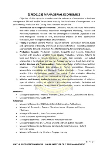
5.2 ASSUMPTIONS OF RETURNS OT SCALEFollowing assumptions are made,1. All inputs can vary except the enterprise2. Workers accurately do their assigned work with provided tools3. There are not technology changes during production4. There is perfect competition5. The output product is measured in quantities.5.3 TYPES OF RETURNS TO SCALEFollowing are the types of return to scale1. Increasing returns to scale2. Constant returns to scale3. Diminishing returns to scaleAccording to the given assumptions with increase in factors of production i.e.,labor and capital following possibilities will be found1. Output may increase in same ratio as input factors2. Output may rise at much higher rate compared to input factors3. Output may increase in very small proportion to increase in inputfactors.It is generally found that the increase in input factors is in fixed proportionsthen output increases in following three different phases.1. INCREASING RETURNS TO SCALE: in this case the output increasing rateis faster than the increasing rate of input factors. For example if theinput factors are doubled or tripled then the output achieved is morethan double or more than triple. Such situation is termed as increasingreturns to scale.FACTOR COMBINATIONS(QUANTALS)1234567TOTAL PRODUCT(QUANTALS)261218242830MARGIANL PRODUCT(QUANTALS)24increasing returns66constant returns64diminishing returns217 P a g eUNIT -3 PRODUCTION ANALYSISBALAJI INSTITUTE OF IT AND MANAGEMENT
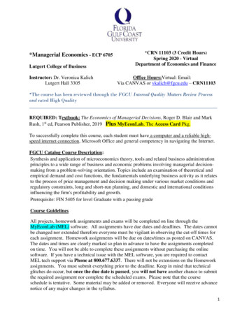
2. CONSTANT RETURN TO SCALE: when the increase in total output exactlyequals to increase in inputs then this situation is termed as constantreturn to scale. Such situation makes marginal returns constant.It is evident from the table above that for 3rd, 4th and 5th units of sale ofproduction the marginal returns remain constant at 6th. This stage II isindicated in figure 3.15 where the portion B to C of CD curve remainsconstant. The portion B to C is horizontal or parallel to scale of productionwhich indicates constant return to scale.Figure: returns to scale3. DIMINISHING RETURNS TO SCALE: such situation indicates arrival ofsaturation stage which does not permit further increases in capacity ofplant. The output increase rate is much less than the increase rate ofinput factors of production. This stage of indicated as stage 3 in figure3.15 which shows a downward trend of returns.6. ECONOMIES DISECONOMIES OF SCALE6.1INTRODUCTION Important information about the processes of production followed byfirm for manufacturing of goods conveyed by the shape of the long-runaverage total cost curve. Economies of scale is when output increases leading to declaiming oflong-run average total cost. Similarly when output increases leading torise of long-run average total cost, it is known as diseconomies of scale.18 P a g eUNIT -3 PRODUCTION ANALYSISBALAJI INSTITUTE OF IT AND MANAGEMENT
6.2:MEANING AND DEFINITION OF ECONOMIES OF SCALE . Economies of scale can be referred to the increasing efficiencies notionof goods production with increasing number of goods produced. Average production cost of goods typically diminishes along withadditional production. This is because fixed costs of production areshared over the additional goods produced.MEANING OF DISECONOMIES OF SCALE Diminishing returns to scale can be observed due to continue expansionof the firm size. When the firm’s expansion goes beyond level growingdiseconomies can be encountered. Economies of production at largescale are canceled by these diseconomies leading to a rise in the averageproduction cost. Diseconomies of scale are not produced generally due to technicalfactors rather these technical factors more likely to limit the sources ofscale economies. In case, inefficiencies are caused because of overlarge size of plant thissituation needs to be avoided. Replication of plant units of smaller sizemay solve the problem in such cases.6.3: KINDS OF ECONOMIES AND DISECONOMIES OF SCALEClassification of the economics of scale and diseconomies of scale canbe done as follows1. Internal economies of scale and internal diseconomies of scale and2. External economies of scale and external diseconomies of scale.19 P a g eUNIT -3 PRODUCTION ANALYSISBALAJI INSTITUTE OF IT AND MANAGEMENT
a)INTERNAL ECONOMIES AND DISECONOMIES OF SCALE1. Technical economics
Managerial Economics by Dominick Salvatore, Ravikesh Srivastava- Oxford University press. Managerial Economics by Hirschey- Cengage Learning. 2 P a g e UNIT -3 PRODUCTION ANALYSIS BALAJI INSTITUTE OF IT AND MANA