Transcription
www.dewesoft.com - Copyright 2000 - 2022 Dewesoft d.o.o., all rights reserved.Fatigue Analysis, Damage calculation,Rainflow counting
What is Fatigue Analysis and Why We Need ItBefore going into the fatigue analysis details, let us consider the following example. Say we wanted to break a metal rod that is not too thick. How would wetackle the task? In a brute-force way like the guy in the picture below or some other way? Well, if we asked a fatigue analysis expert he would probablysuggest us to repeatedly bend both ends of the rod slightly upwards and downwards. And he would be right. The rod would break. Maybe not immediately,maybe not after one hundred repetitions, maybe not after one thousand repetitions, but eventually it would break.How to explain this phenomenon? Let us first describe the physics behind bending the rod. As depicted in the image below, bending induces the stress (σ) inthe cross-section of the rod. Bending the rod upwards induces the positive stress, i.e., compression at the top and tension at the bottom of the cross-section(a), whereas bending the rod downwards causes the negative stress, i.e., tension at the top and compression at the bottom of the cross-section (b). Whenthe rod is in the equilibrium position no stress is induced (c).When bending is repeatedly applied for a su cient period of time microscopic cracks are initiated in the cross-section of the rod. As the bending continuesthese tiny cracks are propagated until they grow to a point where the rod breaks. This phenomenon is called crack propagation.As depicted in the figure below, cracks can propagate in three modes depending on the relative orientation of the load.TensionShearTorsionYou probably don't care much about the broken rod from the example above, right? Well, what if the same rod was a part of a more complex and biggerstructure, such as bridge, an airplane or a train, and its fracture could cause a severe accident with people involved? Clearly, crack propagation poses serious1
problems of both design and analysis in many elds of engineering, especially in civil engineering where safety is of paramount importance. What makescrack propagation even more problematic is that is is very hard to be explicitly detected and measured. Therefore, fatigue analysis engineers typically useimplicit statistical and predictive tools described in the following chapters.2
Fatigue Analysis BasicsIn this chapter, we introduce some basic terms used in fatigue analysis and briefly describe the basics.LoadLoad is defined as any physical quantity that reflects the excitation or the behavior of a system or component over time. The mosttypical loads velocities,accelerations etc.An example of a load signal is depicted in the gure below, showing vertical load measured on a truck transporting gravel. The changes in the mean originatefrom a loaded and unloaded truck, whereas the changes in the standard deviation derived from different road qualities.CycleA half-cycle is a pair of two consecutive extrema in the load signal, going from a minimum to a maximum or vice versa, as depicted in the image 10 below. Afull-cycle is a cycle consisting of two consecutive half-cycles, as depicted in image 11 below.3
The most important cycle characteristics are Range, Amplitude and Mean, defined as follows:Amplitude (Maximum - Minimum) / 2,Range Maximum - Minimum,Mean (Maximum Minimum) / 2.Cycle Counting MethodsCycle counting methods are used to calculate the load spectrum of a load signal, i.e., number of cycles corresponding to each range in a load signal. Anexample of a load spectrum is depicted in the gure below. Typical cycle counting methods are rain ow counting and Markov counting described in thefollowing chapters.FatigueFatigue is the failure mechanism that is caused by repeated load cycles with amplitudes well below the ultimate static material strength. Formally, thefatigue process is divided into three stages:crack initiation,crack propagation,unstable rupture and final fracture.A repeated load applied to a particular object under observation will sooner or later initiate microscopic cracks in the material that will propagate over timeand eventually lead to failure. Fatigue damage is typically cumulative and, therefore, unrecoverable.Fatigue behavior depends on many factors such as:load type,object sizestress/strain concentration and distribution,mean stress/strain,environmental effects,metallurgical factors and material properties,load rate and frequency effects.Fatigue Life Prediction4
Fatigue life prediction is the process of predicting fatigue life of a particular object under observation. According to ASTM fatigue life is de ned as numberof stress cycles that a specimen sustains before failure. Fatigue life prediction is of vital importance in order to assure product quality and safety.DurabilityDurability is the capacity of an item to survive its intended use for a suitable long period of time. Good durability leads to good quality, company pro tabilityand customer satisfaction.5
S-N CurvesGenerally speaking, S-N curves (also known as Wöhler curves) represent statistical models that characterize the material performance. S-N curve isde ned as a graph of the cyclic stress against the logarithmic scale of cycles to failure. The gure below depicts two S-N curves, a red one and a blue one,corresponding to aluminum and steel, respectively. Let us take a closer look at the latter. If the cyclic stress of approximately 45 ksi * is applied to the steelthe failure will occur after 104 cycles, whereas applying lower cyclic stress of approximately 40 ksi will result in failure after 10 5 cycles. Furthermore, at 30 ksithe S-N curve reaches the so-called endurance limit. The endurance limit is the amplitude of the cyclic stress that can be applied to the material withoutcausing fatigue failure. Thus, if the cyclic stress of 30 ksi or less is applied to the steel failure will never occur. On the other hand, at 45 ksi the S-N curvereaches the so-called ultimate stress, defined as the maximum stress a material can withstand.S-N curves are derived from tests on material samples to be characterized (called coupons) where regular sinusoidal stress is applied by a testing machinewhich also counts the number of cycles to failure as depicted in gures (a), (b) and (c) below. This process is known as coupon testing. Each coupon testgenerates a point on the plot though in some cases there is a run-out where the time to failure exceeds that available test period. Analysis of fatigue datarequires techniques from statistics, especially survival analysis and linear regression.6
When designing the components engineers always try to keep the stress amplitudes below the endurance limit, way below the ultimate stress value. Sincethe material never fails below the endurance limit it is safe to be operated at such stress amplitudes.7
Palmgren-Miner RuleThe S-N curves model described in the previous chapter assumes that the material is subjected to a constant amplitude load, i.e., cycles to failurecorrespond to a constant cyclic stress amplitude, as depicted in the image 17 below. The next generalization is to consider a block load, i.e., consecutiveblocks of constant amplitude load, as depicted in the image 18 below.In this case, the Palmgren-Miner damage accumulation hypothesis states that each cycle with amplitude S i uses a fraction 1 / Ni of the total life. Thus thetotal fatigue damage D is given by equation:D iniNiwhere n i is the number of cycles with amplitude S i. Fatigue failure occurs when the damage D exceeds one.Although Palmgren-Miner rule represents a useful approximation model in many circumstances, it has several major limitations:It fails to recognize the probabilistic nature of fatigue.In some circumstances, cycles of low stress followed by high stress cause more damage than the rule predicts. It does not consider the effect of anoverload or high stress which may result in compressive residual stress that may retard crack growth. High stress followed by low stress may have lessdamage due to the presence of compressive residual stress.8
Typical Fatigue Analysis Use-CaseAlthough fatigue analysis covers a very broad range of areas, such as mechanics, physics and statistics, we can simply de ne it as the process ofanalysing, modelling and predicting fatigue behavior. In order to summarize the fatigue analysis basics, let us consider the following example, illustrating avery simple fatigue analysis use-case in the car industry.Suppose that a company, or some company division, is manufacturing drive shafts and a team of engineers is responsible for ensuring they meetperformance, quality and safety requirements. Assuming that preliminary drive shaft tests were already performed and the team is now interested in thelong-term analysis, what would be the next steps?Typically, an engineering team would rst gather as much statistical data as possible, such as target driver group (whether shafts will be used in family cars,trucks etc.), target driver behavior (average driving distance per year, average driving speed etc.), target driving conditions (road conditions, speed limits etc.)and so forth. Afterwards, statistical models describing the target environment would be derived. The models would, consequently, serve in a real-life testing,including real driving in the real environment, with all the required data acquisition taking place, such as measuring load applied to the driver shaft. Finally, thecycle counting methods would be applied to the measured load signals and statistical methods, such as S-N curves or Palmgren-Miner rule, would be usedto check whether load amplitudes exceed the endurance limits of the steel, how often and how much do they exceed it, whether fatigue limit is exceeded,whether Palmgren-Miner damage is exceeded etc. If the results would not comply with the recommended values, the shaft would probably have to undergoadditional modifications and re-engineering.9
Fatigue Analysis in Dewesoft XFatigue Analysis Module supports a wide range of fatigue analysis features and utils. Combined with Dewesoft X it represents a powerful all-in-one fatigueanalysis solution allowing both acquisition and analysis of the fatigue data - everything in a single software package!It is located under Strain, stress Fatigue analysis.The module is organized into three main sections: Preprocessing, Counting methods (Algorithm settings) and Visualization. In fact, section organizationfollows a typical fatigue analysis work ow that starts with the input signal preprocessing, proceeds with the cycle counting and ends with the resultvisualization.Remark:In acquisition mode, only the temporary fatigue analysis results (calculated only over the last block of samples) are displayed. In order to get the actualresults (calculated over all the samples), you need to go to analyse mode and perform recalculation!Each section represents a particular fatigue analysis stage and covers a subset of corresponding methods as follows:1. PreprocessingTurning points filterRainflow filterDiscretization filter2. Counting methodsRainflow counting (ASTM E 1049-85)Markov counting3. VisualizationRange histogramsFrom/to matricesRange/mean matrices4. Damage calculationAccumulated damage (Palmgren-Miner rule)10
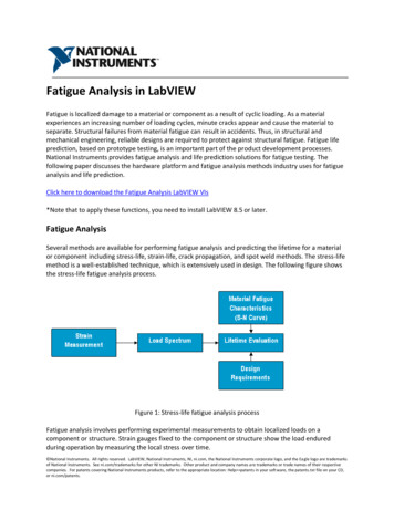
Preprocessing of input signalThe preprocessing section includes turning points filter, rainflow filter and discretization filter.Turning Points FilterTurning points lter detects local extrema, namely turning points, in the load signal. An example of turning point detection is depicted in the gure (a) below.The lter is applied to the input signal by default and cannot be disabled since the Fatigue Analysis Module requires a sequence of turning points as its input(instead of a full load signal).Rainflow FilterRain ow lter (also called the hysteresis lter) removes small oscillations from the signal, as depicted in the gure (b) below. All turning points thatcorrespond to the cycles with the ranges below the given threshold are removed. Higher the threshold, more turning points are ltered out, and vice versa.The rain owltering can signi cantly reduce the number of turning points, which can be of importance for both testing and numerical simulation.Threshold parameter of value T corresponds to the T% of the absolute load signal range.Discretization FilterThe discretization lter divides the range of a load signal into N equidistant bins and assigns each turning point to its closest bin. Figure (c) below depicts anexample where signal ranging from -10 to 10 is discretized into 5 bins. Load signals are typically very stochastic (please refer to the rst gure in the FatigueAnalysis Basics chapter), therefore, discretization is often applied to make them atter and less stochastic. The number of bins is adjusted with the Classcount parameter.Both the rainflow filter and the discretization filter are activated in the Preprocessing section by ticking the appropriate checkbox, as depicted below.11
12
Counting Methods: Markov CountingMarkov counting is one of the most straightforward cycle counting methods. It operates on consecutive pairs of turning points and calculates absoluteranges between them. The method is activated by ticking the Markov counting checkbox in the Algorithm settings section.Figure below depicts an example of Markov counting in action. Clearly, the 6th turning point of the load signal is assigned a value of 5 - 2 3, i.e., theabsolute difference between the 6th and the 5th turning point. Similarly, the 7th turning point is assigned a value of 4 - 5 1, i.e., the absolute differencebetween the 7th and the 6th turning point.When large amplitude cycles (such as the cycle between the 5th and the 8th turning point in the gure above) contain smaller amplitude cycles, Markovcounting fails to detect them. Since large amplitude cycles play an important role in fatigue life, this represents a major drawback of the method.13
Counting Methods: Rainflow CountingRainflow counting is generally accepted as being the best cycle counting method up to date, and has become the industrial de facto standard. It is activatedby ticking the Rainflow counting check box in the Algorithm settings section.The idea behind the method is to detect the hysteresis loops in the load signal, as depicted in the gure below. We'll refer to the hysteresis loops as theclosed cycles. Parts of the signal that do not correspond to the closed cycles are the so-called open cycles or residuals. Simply said, closed cycles andresiduals could be visualized as full-cycles and half-cycles, respectively.As opposed to the Markov counting, which fails to detect large amplitude cycles, the rain ow counting successfully detects them. As depicted in the gurebelow, it detects the large amplitude cycle (2,6) and the small-amplitude cycle (4,5) within.Different rainflow counting standards, such as ASTM, DIN and AFNOR, differ with respect to the treatment of the residuals. In order to be as general aspossible, the Fatigue Analysis Module supports both residual and non-residual mode. When Ignore residuals checkbox in the Additional algorithmsettings section is checked, the residuals are omitted, otherwise, they are included in the results.14
15
VisualizationIn order to graphically represent the results the Fatigue Analysis Module uses the most common visualization techniques used in fatigue analysis: rangehistograms, from/to matrices and range/mean matrices. When an input channel corresponding to a load signal of interest is selected, the following newchannels are mounted:PreprocessingPeak/valley channelRF filter channelDiscretization channelRainflow countingRange histogram channel (2-D)Range/mean matrix channel (3-D)From/to matrix channel (3-D)Markov countingRange histogram channel (2-D)From/to matrix channel (3-D)Remark:The channels marked with 2-D and 3-D correspond to 2-D and 3-D graphs, respectively. The channels corresponding to the Preprocessing sectionrepresent intermediate fatigue analysis results and serve for information purposes only.All the channels are depicted in the screenshot below.16
Visualization: Range HistogramRange histogram is a 2-D graph representing the range distribution of a load signal. An example of a range histogram is depicted in the gure below. The Xaxis and Y-axis of a range histogram correspond to the range and number of cycles, respectively. Thus, if a load signal contained 500 cycles of range 20 and700 cycles of range 40, the entries of (X 20, Y 500) and (X 40, Y 700) would be added to the range histogram.A typical range histogram use-case would be to obtain the range histogram of a signal, rotate it over diagonal (swap the X-axis and Y-axis), overlay acorresponding S-N curve on top and check whether it stays well below the curve.17
Visualization: From/To MatrixFrom/to matrix is a 3D graph representing the cycle distribution of a load signal. An example of a from/to matrix is depicted in the image below.X-axis - From (cycle minimum)Y-axis - To (cycle maximum)Z-axis - Number of cyclesFor example, the image below depicts a cycle ranging from 5 to 10. In this case From and To are assigned the values of 5 and 10, respectively. If a load signalcontained 100 such cycles, entry of (X 5, Y 10, Z 100) would be added to the from/to matrix.18
Visualization: Range/Mean MatrixRange/mean matrix is a 3D graph representing the cycle distribution of a load signal. An example of a range/mean matrix is depicted in the figure below.X-axis - cycle rangeY-axis - cycle meanZ-axis - number of cyclesFor a detailed description of cycle range and cycle mean please refer to Fatigue Analysis Basics chapterFor example, the gure below depicts a cycle ranging from 5 to 10. In this case range and mean are assigned the values of 5 10 - 5 and 7.5 (10 5) / 2,respectively. If a load signal contained 300 such cycles, entry of (X 5, Y 7.5, Z 300) would be added to the range/mean matrix.19
20
Visualization SettingsThe visualization section is organized into three groups: Range, Mean and From/To, as depicted in the screenshot below. Each group controls theappearance of the corresponding graphs. For instance, Range group controls the appearance of the range histograms and the range/mean matrices. Minrange and Max range parameters specify the minimum and maximum of the range axis, whereas the Classes parameter specifies the number of classesthe range is divided into.When the Auto checkbox is ticked Dewesoft automatically calculates Min range and Max range from the input signal. Exactly the same concept goes for theMean and From/To groups as well.Graph appearance can be additionally controlled in the Dewesoft settings window under Extensions Fatigue analysis Settings, as depicted in thescreenshot below.The Ticks parameter controls the position of the graph ticks. When Show ticks at class centers is selected the ticks are displayed exactly at the classcenters, whereas Show ticks at lower-class bounds display them at the lower class bounds, as depicted in the figures (a) and (b) below, respectively.21
22
Additional SettingsAdditional Fatigue Analysis Module settings are located in the Dewesoft settings window under Extensions Fatigue analysis, as depicted in the screenshotbelow.TicksFor the Ticks parameter please refer to the Visualization Settings chapter.Use Hard Drive For CalculationWhen analyzing extremely large data files with the Fatigue Analysis Module the operating system can run out of memory. In order to be as robust as possibleand avoid such scenarios, the module supports a special Hard drive mode. In the hard drive mode all the intermediate data is stored on the hard driveinstead of in the RAM, thus substantially decreasing the memory consumption. The hard drive mode is triggered by ticking the Use hard drive for thecalculation check box. The mode, however, signi cantly reduces the performance and results in higher processing times. Therefore, it should be used only incases where out-of-memory occurs.23
Fatigue analysis measurement exampleIn this chapter, we demonstrate an example of a complete fatigue analysis workflow using the Fatigue Analysis Module and Dewesoft. Let us start with asimple signal, named Stress data, depicted in the screenshot below. The signal is stochastic and has several turning points.First, we activate the Fatigue Analysis Module located under Strain, stress Fatigue analysis. After activating the module the setup screen appears, asdepicted in the image below. We assign an input channel to the module by ticking the Data checkbox on the left-hand side of the screen. We won't be usingany preprocessing, therefore, the Rainflow filtering and Discretization checkboxes are all left unchecked. In order to apply both counting methods, we tick theRainflow counting and Markov counting checkboxes.The next part is the visualization. After ticking all three Auto check boxes Dewesoft automatically assigns the values of 0 and 9 to Min and Max edit boxes.Clearly, since 0 and 9 represent the minimum and maximum of the input signal. For clearer visualization, the Classes parameter is set to 10. Thus, eachclass has width of 1 (9 - 0 1) / 10. Dividing the range into 11 classes, for instance, would not result in the whole number, since (9 - 0 1) / 11 0.91!Finally, we navigate to the Review tab and click the Recalculate button. After recalculation, the result screen is displayed, as depicted in the image below. The24
screen contains ve graphs, i.e., the range histogram and from/to matrix corresponding to the Markov counting, and the range histogram, from/to matrixand range/mean matrix corresponding to the rainflow counting.25
Data ExportThe results obtained in the previous chapter can be optionally exported to a broad range of le formats. Let us, for example, export the data to a text leformat. We navigate to the Export tab, as depicted in the screenshot below, and choose the Text/CSV (*.text, *.csv) from the list of supported le types.After selecting the appropriate channels on the right side of the screen, we click the Export button.When the export has nished the exported text le appears in the Existing les list box. Double-clicking the le opens it in an external text viewer (such asNotepad), as depicted in the screenshot below.Remark:When a full-cycle is detected by rainflow counting it contributes a value of 1 to the total number of cycles, whereas a residual contributes a value of 0.5.Therefore, range histograms and range/mean matrices often contain values such as 0.5, 1.5, 2.5 etc. If we ticked the Ignore residuals check box theresiduals would be ignored and 0.5 values would disappear from the results below.26
27
Damage calculation according to the Palmgren-Miner rule in DewesoftAccording to Miner's Rule, when damage is equal to 1, failure occurs. The definition of failure for a physical part varies. It could mean that a crack hasinitiated on the surface of the part. It could also mean that a crack has gone completely through the part, separating it.In order to make a damage calculation, you need to add an S-N curve in the S-N curve editor.Please make sure that the input units of the signal match the units of the S-N curve. In the S-N curve editor, you can add your own S-N curve, define thename, unit, axis type, and the number of points. When you are done with defining the curve, click the Save button.When the S-N curve is added, go back to the Fatigue analysis module and select option Accumulated damage. When you select this option, you will be ableto go into the S-N curves tab.28
The next step is to go to the S-N curves tab and select the correct S-N curve.Only the overall damage in the defined area of the S-N curve will be calculated. If your stress level or a number of cycles is outside of the predefined area, thedamage will not be added to the overall damage.As seen from the image above for this specific S-N curve, only the damage calculated from the stress levels and cycle numbers inside the orange area willbe added to the overall damage calculation.29
30
Typical Fatigue Analysis Use-Case Although fatigue analysis covers a very broad range of areas, such as mechanics, physics and statistics, we can simply de3ne it as the process of analysing, modelling and predicting fatigue behavior. In order to summarize the fatigue analysis basics, let us consider the following example, illustrating a