Transcription
Deep Learning in the Cloud withMATLAB R2016bBy Stuart Moulder, Tish Sheridan, Amanjit Dulai, Giuseppe RossiniW H I T E PA P E R
Deep Learning in the Cloud with MATLAB R2016bIntroductionYou can use MATLAB to perform deep learning in the cloud using Amazon Elastic Compute Cloud(Amazon EC2) with new P2 instances and data stored in the cloud. Deep learning in the cloud cansave you lots of time if you have big data and models that take hours or days to train.Deep learning is much faster when you can use high performance GPUs for training. If you don’thave a suitable GPU available, you can use the new Amazon EC2 P2 instances to experiment. Try itout using machines with a single GPU, and later scale up to 8 or 16 GPUs per machine to acceleratetraining, using parallel computing to train multiple models at once on the same data. You can compare and explore the performance of multiple deep neural network configurations to look for the besttradeoff of accuracy and memory use.Read the following sections to learn: How to train, test, and explore neural networks for deep learning problems in MATLAB How to scale up deep learning using high performance GPU machines in the Amazon WebServices cloudDeep Learning in MATLABDeep learning is a branch of machine learning that teaches computers to do what comes naturally tohumans and animals: learn from experience. Machine learning algorithms use computational methods to “learn” information directly from data without relying on a predetermined equation as amodel. Deep learning is especially suited for image recognition, which is important for solving problems such as face recognition, motion detection, and many advanced driver assistance technologiessuch as autonomous driving, lane detection, and autonomous parking.Deep learning uses neural networks to learn useful representations of features directly from data.Neural networks combine multiple nonlinear processing layers, using simple elements operating inparallel inspired by biological nervous systems. Deep learning models can achieve state-of-the-artaccuracy in object classification, sometimes exceeding human-level performance. You train modelsusing a large set of labeled data and neural network architectures that contain many layers, usuallyincluding some convolutional layers. Training these models is extremely computationally intensiveand you can usually accelerate training by using a high specification GPU.Figure 1: Example of an image classification modelW H I T E PA P E R 2
Deep Learning in the Cloud with MATLAB R2016bFor this paper, we use a relatively simple network that demonstrates the principles involved. You canuse these same steps to work with larger networks and data-sets. We create a network to classifyimages and show how easy it is to use MATLAB for deep learning, even without extensive knowledgeof advanced computer vision algorithms or neural networks.The goal is to classify images into the correct class. The dataset is the CIFAR-10 dataset, which is anestablished computer-vision dataset used for object recognition. The labeled images were collected byAlex Krizhevsky, Vinod Nair, and Geoffrey Hinton (see Learning Multiple Layers of Features fromTiny Images1, Alex Krizhevsky, 2009). The CIFAR-10 dataset is a commonly used benchmark inmachine learning, because it is complex enough to develop interesting models, but not so large that ittakes days to train. The dataset contains 60,000 32x32 color images in 10 classes, with 6000 imagesper class. Here are the classes in the dataset, showing 10 random images from each class.Figure 2: Classes and example images from the CIFAR-10 dataset1.https://www.cs.toronto.edu/ kriz/learning-features-2009-TR.pdfW H I T E PA P E R 3
Deep Learning in the Cloud with MATLAB R2016bCreate a Deep NetworkNeural Network Toolbox 2 provides simple MATLAB commands for creating the layers of a deepneural network and connecting them together. We expect that to solve the problem, the network willneed a standard set of layers for a convolutional neural network: convolution, pooling, rectified linearunit (ReLU) nonlinearities, and local contrast normalization with a linear classifier on top of it all.The following code shows how to specify and train a single network on your local machine.1. Specify the network layers. The following code creates an array of eleven layers, where the firstlayer receives input images and the last layer classifies the image by returning the category.layers [imageInputLayer([32 32 ationLayer()];To learn more about any of the layers, see the Neural Network Toolbox documentation3.2. 3. https://www.mathworks.com/help/nnet/W H I T E PA P E R 4
Deep Learning in the Cloud with MATLAB R2016b2. Specify training options to define the training method and its parameters. The options here willtrain for 30 epochs with a learning rate of 0.001, then reduce the learning rate by a factor of 10,and continue training for another 10 epochs. Each epoch means one full training cycle on thewhole training set. Verbose set to true displays the progress of training.% Define the training optionsoptions trainingOptions(‘sgdm’, .‘InitialLearnRate’, 0.001, .‘LearnRateSchedule’, ‘piecewise’, .‘LearnRateDropFactor’, 0.1, .‘LearnRateDropPeriod’, 30, .‘L2Regularization’, 0.004, .‘MaxEpochs’, 40, .‘MiniBatchSize’, 100, .‘Verbose’, true);3. Supply the set of labeled training images to imageDatastore, specifying where you have savedthe data. You can use an imageDatastore to efficiently access all of the image files. imageDatastore is designed to read batches of images for faster processing in machine learning andcomputer vision applications. imageDatastore can import data from image collections that aretoo large to fit in memory.% Define the training dataimdsTrain ,’foldernames’);The CIFAR-10 images are split into a set to use for training and a second set to use for testing. Thetraining set in this example is in a local folder called ‘cifar-10-32-by-32/cifar10Train’.To get the data, see Appendix - Prepare the CIFAR-10 data.W H I T E PA P E R 5
Deep Learning in the Cloud with MATLAB R2016b4. To train the network, use the trainNetwork function:net trainNetwork(imdsTrain,layers,options);The result is a fully trained network that you can use to classify new images.Test the NetworkAfter you create a fully trained network, you can use it to classify a new set of images and measurehow accurate it is. The following code tests the accuracy of classification using the test set. The accuracy score is the percentage of correctly classified images using the test set.% Define the testing dataimdsTest ’foldernames’);% Measure the accuracyyTest classify(net,imdsTest);accuracy (sum(yTest imdsTest.Labels) / numel(imdsTest.Labels));Try Different ModelsHaving trained one network, we want to see whether modifying this network can improve the accuracy of the model in classifying images correctly. There are many ways to configure your network, butfor this example we investigate changing the number of filters, filter size, pooling size, and addingadditional convolutional layers. The convolutional and fully connected layers add learnable parameters, which might increase accuracy but will increase memory usage. When we have a selection oftrained models to compare, we can assess them to choose the best tradeoff of accuracy and memoryfootprint. For the complete MATLAB script training the networks in parallel, seeAppendix – MATLAB Code.Training all these different models on just a desktop PC is going to take a long time. Instead, we wantto make use of a high specification multi-GPU machine. Amazon can provide us with suitablemachines on demand using their new P2 instances. In the following sections, you can learn how toreserve a P2 instance, how to connect to the data, and then how to simultaneously train models in thecloud.W H I T E PA P E R 6
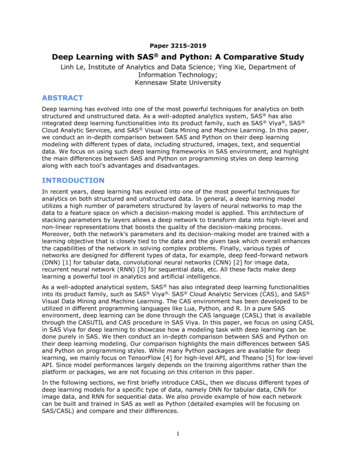
Deep Learning in the Cloud with MATLAB R2016bScale Up to Deep Learning in the CloudTo try out deep learning in the cloud, you need: MATLAB R2016b, Neural Network Toolbox, Parallel Computing Toolbox A MathWorks Account Access to MATLAB Distributed Computing Server for Amazon EC24 . An Amazon Web Services accountConnecting to Amazon EC2 Using MathWorks Cloud CenterAmazon Elastic Compute Cloud (Amazon EC2) is a web service which you can use to set up computecapacity and storage in the cloud. Amazon EC2 is ideally suited for the intensive computationaldemands and large datasets found in deep learning. By using Amazon EC2, you can economicallyscale up your computing resources and gain access to domain-specific hardware. The newAmazon EC2 P25 instances are specifically designed for compute-intensive applications, providing upto 16 NVIDIA Tesla K80 GPUs per machine. You can use a single GPU to take advantage of the parallel nature of neural networks, dramatically reducing the time required to train a single model. Youcan use multiple GPUs to try more models, allowing you to train multiple models simultaneously.You can scale up beyond the desktop, and scale in a flexible way without requiring any long-termcommitment.MathWorks Cloud Center is a web application for creating and accessing compute clusters in theAmazon Web Services cloud for parallel computing with MATLAB. You can access a cloud clusterfrom your client MATLAB session like any other cluster in your own onsite network. To learn more,see MATLAB Distributed Computing Server for Amazon EC26.For instructions to help you set up your credentials and then create a new cluster, see Create andManage Clusters7 in the Cloud Center documentation. The main steps are:1. Log in to Cloud Center8 using your MathWorks account email address and password.2. Click User Preferences and follow the on-screen instructions to set up your Amazon Web Services(AWS) credentials. For help, see the Cloud Center documentation: Set Up Your Amazon WebServices (AWS) Credentials93. To create a cluster of Amazon EC2 instances, click Create a Cluster.4. Choose the settings as shown in the following screenshot. To create a cluster suitable for deeplearning, you must configure the Machine Type to include high performance GPUs. Choose amachine type with multiple GPUs per machine to train multiple networks in parallel.4.5.6.7.8.9.W H I T E PA P E enter/ug/cloud-computing-console.html#butnm c-1 7
Deep Learning in the Cloud with MATLAB R2016bFigure 3 Cloud Center: Create a cluster with multiple GPUs5. Click create a new key so that you can download and save the SSH key for root access. You willneed this to log in using SSH and set up your cluster to access the data in a later step.6. Click Create Cluster.7. To access your cluster from MATLAB, use Parallel Discover Clusters to search for yourAmazon EC2 clusters. When you select the cluster, the wizard automatically sets it as yourdefault cluster.8. On the MATLAB Home tab, select Parallel Parallel Preferences, and set Preferred number ofworkers to 16.Check if your cluster is online, either from Cloud Center, or from within MATLAB by creating a cluster instance and displaying details:cluster parcluster();disp(cluster);W H I T E PA P E R 8
Deep Learning in the Cloud with MATLAB R2016bBy default, if the cluster is left idle for too long it automatically shuts down to avoid incurringunwanted expense. If your cluster has shut down, bring it back online either from Cloud Center byclicking Start Up, or from MATLAB by entering:start(cluster);After your cluster is online, query the GPU device of each worker:wait(cluster)spmddisp(gpuDevice());endThis returns details of the GPU device visible to each worker process in your cluster. The spmd blockautomatically starts the workers in a parallel pool, if you have default preferences. The first time youcreate a parallel pool on a cloud cluster can take several minutes.You can start or shut down the parallel pool using the Parallel Pool menu in the bottom left of theMATLAB desktop.To learn more about using parallel pools, see the Parallel Pools documentation10.Using Data in Amazon EBS VolumesIn this example, we choose to store our data in Amazon Elastic Block Store (Amazon EBS). AmazonEBS is a service which provides flexible, scalable, and durable storage in the cloud. You can use EBSvolumes with your Amazon EC2 instances. To create a volume, we used the AWS Console to create a100GB general purpose solid state drive (SSD gp2). This is Amazon Web Service’s default volume typeand is suitable for most applications.AWS provides many options to configure your storage, including volume type and size. The optimalchoice of storage depends on your Amazon EC2 instance type and the read/write requirements ofyour application. To learn more about the different Amazon EBS volumes available, see theAmazon EBS Volume Types documentation11.You must attach and mount the EBS volume for your cluster. For instructions, seeAppendix – Transfer Data to EBS Volume.10. ools.html11. /EBSVolumeTypes.htmlW H I T E PA P E R 9
Deep Learning in the Cloud with MATLAB R2016bTo access your training data in MATLAB, you can simply create an imageDatastore pointing tothe appropriate location. This example used /mnt/datastore.parfor ii 1:numNetworksToTrain% Define the Amazon EBS storage training data (must run on thecluster)imdsTrain 2/cifar10Train’, ��foldernames’);.% SEE APPENDIX FOR COMPLETE SCRIPTYou need to run this imageDatastore command inside a parallel for-loop because the data is onlyvisible to the workers on the cluster. You can see this command inside the entire parfor loop in thenext section. If you run the code in your local MATLAB client and not in parallel, it will errorbecause the folder only exists on the cluster.Note: when your cluster shuts down, the Amazon EBS volume is automatically detached. Your data isretained, but when you want to use it again in an online cluster, you must repeat the steps to attachand mount the volume.Deep learning Using MATLAB and Amazon EC2Having used MathWorks Cloud Center and Amazon EC2 to access sufficient compute capacity, andAmazon EBS Volumes to store and access our dataset, we now want to quickly train the optimal network for our problem. In this example we are searching for the network which gives the best balancebetween high classification accuracy and low memory footprint. We test 16 different networks, andfor each model store the classification accuracy and memory footprint. We investigated changing thenumber of filters, filter size, pooling size, and adding additional convolutional layers.Training and validating each model is an independent process, so you can use parallel computing tocompute multiple models simultaneously. To do this, you can iterate over the different models using aparfor loop. A parfor loop executes loop iterations in parallel on MATLAB workers in the parallelpool and parfor distributes the work among as many workers as you have available in the pool.W H I T E PA P E R 10
Deep Learning in the Cloud with MATLAB R2016bFollowing is the part of the MATLAB script that trains and tests the 16 different networks in parallel.To see the entire script including the supporting functions, see Appendix – MATLAB Code.%% Train all network configurationsparfor idx 1:numNetworksToTrain% Get the network configuration to train on this workerlayers networks{idx};% Load the training and test dataimdsTrain �foldernames’);imdsTest ��IncludeSubfolders’,true, .‘LabelSource’,’foldernames’);% Train the networknet trainNetwork(imdsTrain,layers,options);% Record the memory footprint for this networkmemoryFootprints(idx) getMemoryFootprint(net);% Record the accuracy for this networkyTest classify(net,imdsTest);accuracies(idx) sum(yTest imdsTest.Labels) / numel(imdsTest.Labels);% Save the networktrainedNetworks{idx} net;end% SEE APPENDIX FOR COMPLETE SCRIPTW H I T E PA P E R 11
Deep Learning in the Cloud with MATLAB R2016bResultsThe following plot shows the results of training, validating, and characterizing the 16 different chosennetworks. Using these results, we can identify which network to use depending on our accuracy andmemory requirements. The best model is a tradeoff choice. Memory footprint might be an importantconsideration, for example if you need the final network to run on an embedded processor in a car.Figure 4: Classification accuracy versus memory footprint for the different model parameters testedThe graph shows accuracy against memory footprint. The red line shows the networks along thePareto front – these are the optimal choices for accuracy against memory. Points that do not lie alongthe Pareto front all have worse accuracy or memory use. The best model is one of the points on thePareto front, and which to choose depends on memory constraints and acceptable accuracy.The memory footprint of a neural network is proportional to the number of learnable parameters,which come from the convolutional and fully connected layers. You might assume that more learnableparameters lead to better performance and so you should choose the largest model that will fitmemory constraints. However, sometimes larger models can have worse performance than smallermodels. More learnable parameters can sometimes lead to overfitting, especially if a large amount ofthe learnable parameters are in the final fully connected layer. You can use Dropout to mitigate this.W H I T E PA P E R 12
Deep Learning in the Cloud with MATLAB R2016bA larger model can also take longer to converge, and may require more epochs of training than asmaller model.We investigated changing the number of filters, filter size, pooling size, and adding additional convolutional layers. To see all the settings, examine the code in the appendix. These types of parametersweeps are very important for finding the best performance, but training each network in series canbe prohibitively slow. Using a parallel pool gives multiple workers, but on a single GPU machine competition between workers for GPU resources limits the performance of each worker, reducing the parallel performance of the parfor loop. As described earlier, you can use MathWorks Cloud Center tostart a cluster on Amazon EC2 with the necessary software and GPU resources to massively parallelize this sort of parameter sweep with MATLAB.By creating a cluster using an Amazon EC2 p2.16xlarge instance with 16 GPUs, you can get up to 16workers on a single machine, each with their own processor thread and GPU. We now repeat thesame model parameter sweep, but using a different number of workers each time. Below we show thespeedup as a function of the number of workers, defining speedup as the number of networks trainedper unit time.Figure 5 Speed up factor versus the number of workers for P2.16xlarge Amazon EC2 instanceThese results show that the parallel performance of these instances scales well with the number ofworkers. You can get more workers and more GPUs by using Cloud Center to run MATLAB on powerful Amazon EC2 machines that speed up your deep learning calculations.W H I T E PA P E R 13
Deep Learning in the Cloud with MATLAB R2016bConclusionsIn this paper we show how you can use MATLAB R2016b to explore the performance of various deepneural network configurations, with accelerated training using the computing power of Amazon EC2and cloud data storage. The code provides a worked example showing how to train a network to classify images, and use it to classify a new set of images plus measure the accuracy of the classificationand its memory footprint. You can use a parfor loop to train multiple models simultaneously by distributing the work among as many MATLAB workers as you have available, and you can switch toprocessing on a cluster without leaving your client MATLAB.Useful Links:For more information, see the following resources: mathworks.com/discovery/deep-learning.htmlCentral resource for deep Learning with MATLAB rks.htmlNeural Network Toolbox documentation on essential tools for deep learning Learning Multiple Layers of Features from Tiny Images12, Alex Krizhevsky, 2009About the CIFAR-10 dataset -computing-on-the-cloud/ https://aws.amazon.com/console/See the appendices for MATLAB code and steps for setting up data on a cluster.12. https://www.cs.toronto.edu/ kriz/learning-features-2009-TR.pdfW H I T E PA P E R 14
Deep Learning in the Cloud with MATLAB R2016bAppendix – MATLAB CodeThe following MATLAB code trains the selection of neural networks in parallel, and generates theplot shown in the Results section. The supporting functions define which parameters to sweep in thedifferent networks and compute the memory footprints of the trained networks.% Create the 16 different network configurations we want to testnetworks createTestNetworks();% Allocate variables for networks, memory footprints, and accuracynumNetworksToTrain numel(networks);trainedNetworks cell(numNetworksToTrain,1);memoryFootprints zeros(numNetworksToTrain,1);accuracies zeros(numNetworksToTrain,1);% Define the training options% For a quick test, try setting MaxEpochs to 1.options ,false);% Start parallel pool of 16 workersp gcp(‘nocreate’);if isempty(p)parpool(16);elseif p.NumWorkers 16delete(p);W H I T E PA P E R 15
Deep Learning in the Cloud with MATLAB R2016bparpool(16);end%% Train all network configurationsdisp(‘Starting parallel training .’);parfor idx 1:numNetworksToTrain% Get the network configuration to train on this workerlayers networks{idx};% Load the training and test dataimdsTrain �foldernames’);imdsTest foldernames’);% Train the networknet trainNetwork(imdsTrain,layers,options);% Record the memory footprint for this networkmemoryFootprints(idx) getMemoryFootprint(net);% Record the accuracy for this networkyTest classify(net,imdsTest);accuracies(idx) sum(yTest imdsTest.Labels) / numel(imdsTest.Labels);% Save the networktrainedNetworks{idx} net;enddisp(‘Finished parallel training .’);W H I T E PA P E R 16
Deep Learning in the Cloud with MATLAB R2016b%% Plot the memory footprints against the (‘Accuracy against Memory Footprint’);xlabel(‘Memory Footprint in -------function networks createTestNetworks()% Network parameters to iterate overnumFilters1Values [20 32];filterSizeValues [5 3];poolSizeValues [3 2];useExtraLayerValues [0 1];numNetworksToTrain 16;numFilters1Sweep eSweep eep rSweep s cell(numNetworksToTrain,1);for idx 1:numNetworksToTrainnumFilters1 numFilters1Sweep(idx);numFilters2 numFilters1 * 2;filterSize filterSizeSweep(idx);poolSize poolSizeSweep(idx);useExtraLayer useExtraLayerSweep(idx);if useExtraLayerW H I T E PA P E R 17
Deep Learning in the Cloud with MATLAB R2016bextraLayer ��,0.75,’K’,1)];elseextraLayer [];endnetworks{idx} [imageInputLayer([32 32 n memoryInBytes getMemoryFootprint(net)% Compute the total memory footprint of a trained networkW H I T E PA P E R 18
Deep Learning in the Cloud with MATLAB R2016blayers net.Layers;numParameters zeros(size(layers));for idx 1:numel(net.Layers)switch class(net.Layers(idx))case umParameters(idx) numImageInputParameters(net.case );numParameters(idx) num2dConvolutionParameters(net.case ));numParameters(idx) ters(idx) 0;endend% Each value will be 4 bytes in single precisionmemoryInBytes 4*sum(numParameters);endfunction numParameters ering(layer))numParameters prod(layer.InputSize);elsenumParameters 0;endendfunction numParameters num2dConvolutionParameters(layer)W H I T E PA P E R 19
Deep Learning in the Cloud with MATLAB R2016bnumParameters (prod(layer.FilterSize)*layer.NumChannels 1) * layer.NumFilters;endfunction numParameters numFullyConnectedParameters(layer)numParameters (layer.InputSize 1)*layer.OutputSize;endfunction tf layerUsesZeroCentering(layer)tf pendix – Transfer Data to EBS VolumeIf your application needs many small files, which is common in deep learning image recognitionapplications, the fastest way to access your data on the cluster is to attach and mount Amazon ElasticBlock Store (EBS) volumes.To get your data onto your cluster, use Cloud Center, the AWS console, and SSH to create and mountan EBS volume.1. In Cloud Center, create a cluster and create a new SSH key for root access.See console.html2. Use the Amazon Web Services (AWS) Console to create an Amazon EBS volume.See https://aws.amazon.com/console/a. In AWS, select EC2.b. In the top navigation bar, select the same region as your cluster (eg US-East, EU-West, etc.).You can only attach a volume to Amazon EC2 clusters from the same region.c. Under ELASTIC BLOCK STORE, choose Volumes, and click Create Volume.d. Choose a volume type. For example, the 100GB general purpose solid state drive (SSD gp2) isAmazon EBS’s default volume type and is suitable for most applications. Amazon providesmany options and the optimal choice depends on your application’s read/write requirements.e. Select the Availability Zone that matches your Amazon EC2 instances. For example, eu-west1b. You can check the zone of your cluster on the Instances pane in the EC2 console.For help see e/ebs-creating-volume.html3. Use the Amazon Web Services (AWS) Console to attach your Amazon EBS volume.a. Select your created volume and chose Actions Attach Volume.b. Enter the name or ID of your Amazon EC2 instance, or simply select it from the drop downmenu.W H I T E PA P E R 20
Deep Learning in the Cloud with MATLAB R2016bc. Leave the default device name.d. Click Attach. For help attaching volumes, refer to Amazon Web Service’s instructions inAttaching an Amazon EBS Volume13.4. To make the volume available for the cluster to use, you must mount the volume.On Windows:a. Use Putty Key Generator to import and save your SSH root access key.b. Use Putty to connect to your cluster using SSH. Your user name is ubuntu and the host nameis the MATLAB Job Scheduler Host name, that you can look up in Cloud Center on the ClusterSummary. This is an example: ws.comFor more help on connecting to the cluster machine from Windows,see /putty.html.On Linux:a. Set permissions on your SSH root access key.[user ] % chmod 600 root key.pemb. Connect to your cluster using SSH, the root access key, and the MATLAB Job Scheduler Hostname of your cluster, as shown in this example:[user ] % ssh -i root key.pem ws.com5. Create a mount point directory for your volume. This determines the location where you will readand write to your volume after it is mounted. Do not specify /mnt/matlab or /mnt/persisted,because Cloud Center creates these volumes. For example, we specified /mnt/datastore:[ubuntu ] % sudo mkdir -p -m a rwx /mnt/datastore6. Use the lsblk command to find the disk drive cor
Deep Learning in MATLAB Deep learning is a branch of machine learning that teaches computers to do what comes naturally to humans and animals: learn from experience. . Neural Network Toolbox 2 provides simple MATLAB commands for creating the layers of a deep neural network and connecting them together. We expect that to solve the problem .