Transcription
Paper 3215-2019Deep Learning with SAS and Python: A Comparative StudyLinh Le, Institute of Analytics and Data Science; Ying Xie, Department ofInformation Technology;Kennesaw State UniversityABSTRACTDeep learning has evolved into one of the most powerful techniques for analytics on bothstructured and unstructured data. As a well-adopted analytics system, SAS has alsointegrated deep learning functionalities into its product family, such as SAS Viya , SAS Cloud Analytic Services, and SAS Visual Data Mining and Machine Learning. In this paper,we conduct an in-depth comparison between SAS and Python on their deep learningmodeling with different types of data, including structured, images, text, and sequentialdata. We focus on using such deep learning frameworks in SAS environment, and highlightthe main differences between SAS and Python on programming styles on deep learningalong with each tool’s advantages and disadvantages.INTRODUCTIONIn recent years, deep learning has evolved into one of the most powerful techniques foranalytics on both structured and unstructured data. In general, a deep learning modelutilizes a high number of parameters structured by layers of neural networks to map thedata to a feature space on which a decision-making model is applied. This architecture ofstacking parameters by layers allows a deep network to transform data into high-level andnon-linear representations that boosts the quality of the decision-making process.Moreover, both the network’s parameters and its decision-making model are trained with alearning objective that is closely tied to the data and the given task which overall enhancesthe capabilities of the network in solving complex problems. Finally, various types ofnetworks are designed for different types of data, for example, deep feed-forward network(DNN) [1] for tabular data, convolutional neural networks (CNN) [2] for image data,recurrent neural network (RNN) [3] for sequential data, etc. All these facts make deeplearning a powerful tool in analytics and artificial intelligence.As a well-adopted analytical system, SAS has also integrated deep learning functionalitiesinto its product family, such as SAS Viya , SAS Cloud Analytic Services (CAS), and SAS Visual Data Mining and Machine Learning. The CAS environment has been developed to beutilized in different programming languages like Lua, Python, and R. In a pure SASenvironment, deep learning can be done through the CAS language (CASL) that is availablethrough the CASUTIL and CAS procedure in SAS Viya. In this paper, we focus on using CASLin SAS Viya for deep learning to showcase how a modeling task with deep learning can bedone purely in SAS. We then conduct an in-depth comparison between SAS and Python ontheir deep learning modeling. Our comparison highlights the main differences between SASand Python on programming styles. While many Python packages are available for deeplearning, we mainly focus on TensorFlow [4] for high-level API, and Theano [5] for low-levelAPI. Since model performances largely depends on the training algorithms rather than theplatform or packages, we are not focusing on this criterion in this paper.In the following sections, we first briefly introduce CASL, then we discuss different types ofdeep learning models for a specific type of data, namely DNN for tabular data, CNN forimage data, and RNN for sequential data. We also provide example of how each networkcan be built and trained in SAS as well as Python (detailed examples will be focusing onSAS/CASL) and compare and their differences.1
BASIC CAS LANGUAGEThe CAS Language is available through SAS Viya under the CAS and CASUTIL procedure. Ina SAS Studio environment that is connected to SAS Viya, the users can initiate a CASsession simply with running:cas;The user can also give the CAS session a name, for example:cas casauto;begins a CAS session named “𝑐𝑎𝑠𝑎𝑢𝑡𝑜”. A successfully initiated session gives a message thatis showed in Figure 1.Figure 1. Logs from a Successfully Initialized CAS SessionA simple way to load data into a CAS session is to create a CAS library (𝑐𝑎𝑠𝑙𝑖𝑏) referenceand use it to store data with a data step like a normal lib name. For example:caslib all assign;libname inmem cas caslib casuser;data inmem.train;set dnntest.train;data inmem.test;set dnntest.test;In details, the piece of code above first makes all cas libraries available to the current SASsession. It then creates a library reference named 𝑖𝑛𝑚𝑒𝑚 that links to the caslib 𝑐𝑎𝑠𝑢𝑠𝑒𝑟.Then, two data steps are used to save the 𝑡𝑟𝑎𝑖𝑛 and 𝑡𝑒𝑠𝑡 datasets from the 𝑑𝑛𝑛𝑡𝑒𝑠𝑡 library tothe caslib 𝑐𝑎𝑠𝑢𝑠𝑒𝑟. Both library references and the datasets they contain can be seen in SASStudio, as showed in Figure 2.Figure 2. Datasets in a CAS Library and its Library ReferenceFurther steps of conducting analyses are done through “actions” in the CAS procedure. Inshort, an action is similar to a statement in other SAS procedures. CAS actions are dividedinto action sets of based on their use cases. The general syntax is to call the CASprocedure, then call the actions along with defining their required parameters. The followingsnippet of codes:2
proc cas;session casauto;table.tableInfo /caslib "casuser";name "train";run;quit;invokes the 𝑡𝑎𝑏𝑙𝑒𝐼𝑛𝑓𝑜 action from the action set 𝑡𝑎𝑏𝑙𝑒 in the CAS procedure. The parametersof the action in this case set the target caslib location to 𝑐𝑎𝑠𝑢𝑠𝑒𝑟 and the target dataset to𝑡𝑟𝑎𝑖𝑛. The result of this snippet can be seen in Figure 3.Figure 3. Result of the 𝒕𝒂𝒃𝒍𝒆𝑰𝒏𝒇𝒐 ActionIn the next sections, we review the theory if DNN, CNN, and RNN, then show how they canbe built in CASL as well as Python.DEEP LEARNING IN CASLDEEP FEED-FORWARD NETWORKThe simplest form of a deep network is a deep feed-forward network or a deep neuralnetwork (DNN). Mathematically, let 𝐻𝑖 , 𝑊𝑖 , and 𝑏𝑖 denote the output, the weight matrix, andthe bias vector of hidden layer 𝑖 respectively, then𝐻𝑖 𝜎(𝑊𝑖 𝐻𝑖 𝑏𝑖 )(1)with 𝜎( ) being an activation function. The most commonly used activation functions are1sigmoid (𝜎(𝑥) ), hyperbolic tangent (𝜎(𝑥) tanh(𝑥)), or rectified linear function1 exp( 𝑥)(ReLU) (𝜎(𝑥) max(0, 𝑥)). The input layer can be denoted as 𝐻0 𝑋 (𝑗) with 𝑋 (𝑗) being datainstance 𝑗, and its output is 𝑦̂ 𝑠(𝑊𝑘 𝐻𝑘 𝑏𝑘 ) with 𝑘 being the number of hidden layers, and𝑠( ) being an output function. 𝑠( ) is selected based on the given task, for example, in amultilabel classification problem 𝑠( ) is often the SoftMax function which output a vector withexp(𝑥𝑖 )the 𝑖 𝑡ℎ dimension being 𝑠𝑖 (𝑥) . In a regression problem, 𝑠( ) is an identity function (exp(𝑥𝑗 ))(𝑠(𝑥) 𝑥). Overall, the computation from a data instance 𝑋 (𝑖) to its prediction 𝑌 (𝑖) in a DNN of𝑘 hidden layers can be represented as follows𝐻0 𝑋 (𝑖)𝐻1 𝜎(𝑊0 𝐻0 𝑏0 )𝐻2 𝜎(𝑊1 𝐻1 𝑏1 ) 𝐻𝑘 𝜎(𝑊𝑘 1 𝐻𝑘 1 𝑏𝑘 1 )𝑦 (𝑖) 𝑠(𝑊𝑘 𝐻𝑘 𝑏𝑘 )DNNs are usually trained to minimize a predefined cost function 𝐿, varied by the tasks,using gradient descent. Parameters in layer 𝑖 of the DNN are updated by3(2)
𝐿 𝑊𝑖 𝐿𝑏𝑖 𝑏𝑖 𝛼 𝑏𝑖𝑊𝑖 𝑊𝑖 𝛼 (3)With 𝛼 being a selected learning rate (a positive scalar, normally smaller than 1). 𝐿 isselected based on the given task, for example Binary Cross-Entropy or Negative LogLikelihood for classification, and Mean Squared Error for regression. In recent years, theReLU activation function is preferred over others since it solves the gradient vanishingproblem (gradients approach 0 when being passed to deeper layers with respect to theoutput layer).In CAS, a DNN is built layer by layer. In other words, the users first generate an emptynetwork where new layers are added sequentially. In general, the required parameters foreach layer are its type, input, output, number of hidden neurons, and activation function. InCAS, the basic actions for building, training, and scoring a DNN are 𝑏𝑢𝑖𝑙𝑑𝑀𝑜𝑑𝑒𝑙, ���𝑖𝑛, and 𝑑𝑙𝑆𝑐𝑜𝑟𝑒, which are available in the 𝑑𝑒𝑒𝑝𝐿𝑒𝑎𝑟𝑛 action set. Additionally, the𝑚𝑜𝑑𝑒𝑙𝐼𝑛𝑓𝑜 action in the same action set can be used to obtain information about an existingnetwork. The code snippet below creates an empty DNN then adds an input layer, twohidden layers, and one output layer to it:proc cas;session casauto;deepLearn.buildModel /modelTable {name "DNN",replace TRUE}type "DNN";run;deepLearn.addLayer /layer {type "INPUT"}modelTable {name "DNN"}name "data";run;deepLearn.addLayer /layer {type "FC"n 50act 'relu'init 'xavier'}modelTable {name "DNN"}name "dnn1"srcLayers {"data"};run;deepLearn.addLayer /layer {type "FC"n 50act 'relu'init 'xavier'}modelTable {name "DNN"}name "dnn2"srcLayers {"dnn1"};run;deepLearn.addLayer /layer {type "output"act 'softmax'4
init 'xavier'}modelTable {name "DNN"}name "outlayer"srcLayers {"dnn2"};run;quit;First, the 𝑏𝑢𝑖𝑙𝑑𝑀𝑜𝑑𝑒𝑙 action initialize an empty DNN and links it to a new CAS dataset named𝐷𝑁𝑁. The 𝑟𝑒𝑝𝑙𝑎𝑐𝑒 𝑇𝑅𝑈𝐸 argument specifies to overwrite the DNN dataset if it has alreadyexisted, and the 𝑡𝑦𝑝𝑒 𝐷𝑁𝑁 specifies that the network is a deep feed-forward network.Next, the 𝑎𝑑𝑑𝐿𝑎𝑦𝑒𝑟 action is used to add one input layer, two hidden layer, and one outputlayer to the empty network. The 𝑙𝑎𝑦𝑒𝑟 argument of 𝑎𝑑𝑑𝐿𝑎𝑦𝑒𝑟 specifies the adding layer’sparameters such as layer type (in this case, we have 𝑖𝑛𝑝𝑢𝑡, 𝐹𝐶 – fully connected, and𝑜𝑢𝑡𝑝𝑢𝑡), number of hidden neurons in the layer (𝑛 50), activation function (𝑎𝑐𝑡 ’𝑟𝑒𝑙𝑢’), andthe weight initialization method (𝑖𝑛𝑖𝑡 ’𝑥𝑎𝑣𝑖𝑒𝑟’). Three other important arguments of the𝑎𝑑𝑑𝐿𝑎𝑦𝑒𝑟 action are 𝑚𝑜𝑑𝑒𝑙𝑇𝑎𝑏𝑙𝑒, 𝑛𝑎𝑚𝑒 and 𝑠𝑟𝑐𝐿𝑎𝑦𝑒𝑟𝑠 which defines the target network, thename of the adding layer, and the layer that act as the input of the adding layer,respectively. In this case, the names of the four layers are “𝑑𝑎𝑡𝑎”, “𝑑𝑛𝑛1”, “𝑑𝑛𝑛2”, and“𝑜𝑢𝑡𝑙𝑎𝑦𝑒𝑟”; they are sequentially connected: 𝑑𝑎𝑡𝑎 𝑑𝑛𝑛1 𝑑𝑛𝑛2 𝑜𝑢𝑡𝑙𝑎𝑦𝑒𝑟. The results fromthe 𝑏𝑢𝑖𝑙𝑑𝑀𝑜𝑑𝑒𝑙 and 𝑎𝑑𝑑𝐿𝑎𝑦𝑒𝑟 action are showed in Figure 4.Figure 4. Results from Actions to Build a DNNAfter adding layers to the network, the action 𝑚𝑜𝑑𝑒𝑙𝐼𝑛𝑓𝑜 can be used to show the networkarchitecture:proc cas;session casauto;deepLearn.modelInfo /modelTable {name "DNN"};run;quit;The result of the 𝑚𝑜𝑑𝑒𝑙𝐼𝑛𝑓𝑜 action can be seen in Figure 5.Figure 5. Result of the modelInfo ActionFinally, the network is trained and scored with the 𝑑𝑙𝑇𝑟𝑎𝑖𝑛 and 𝑑𝑙𝑆𝑐𝑜𝑟𝑒 actions. The codesnippet below trains the network using the Adam method [6] in 10 iterations (epochs) in the𝑡𝑟𝑎𝑖𝑛 dataset then scores the trained network in the 𝑡𝑒𝑠𝑡 dataset.5
proc cas;session casauto;deepLearn.dlTrain /inputs odelTable {name "DNN"}modelWeights {name "DNNWeights",replace TRUE}nThreads 1optimizer {algorithm {method "ADAM",lrPolicy 'step',gamma 0.5,beta1 0.9,beta2 0.999,learningRate 0.1},maxEpochs 10,miniBatchSize 1}seed 54321table {caslib "casuser",name "train"}target "y"nominal "y";run;deepLearn.dlScore /initWeights {name "DNNWeights"}modelTable {name "DNN"}table {caslib "casuser",name "test"};run;quit;Important arguments of the 𝑑𝑙𝑇𝑟𝑎𝑖𝑛 action include the input variables (𝑖𝑛𝑝𝑢𝑡𝑠 ), thenetwork to train (𝑚𝑜𝑑𝑒𝑙𝑇𝑎𝑏𝑙𝑒 ), the dataset to store the trained weights (𝑚𝑜𝑑𝑒𝑙𝑊𝑒𝑖𝑔ℎ𝑡𝑠 ) –which will be created during training, the training data (𝑡𝑎𝑏𝑙𝑒 ), and the target variable(𝑡𝑎𝑟𝑔𝑒𝑡 ). In this case, the network is trained for a classification task, so we add the𝑛𝑜𝑚𝑖𝑛𝑎𝑙 argument. In the 𝑑𝑙𝑆𝑐𝑜𝑟𝑒 action, the users specify the weight table and networktable, and the target scoring data. The result of the two actions can be seen in Figure 6.6
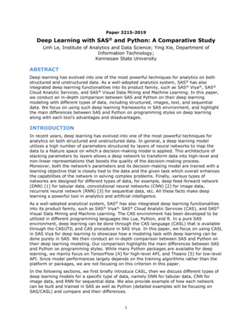
Figure 6. Results from the dlTrain and dlScore ActionsCONVOLUTIONAL NEURAL NETWORKThe CNN architecture uses a set of filters that are slide through the pixels of each inputimage to generate feature maps, which allows features to be detected regardless of theirlocations in the image. The feature maps output by a convolutional layer are usually furthersubsampled to reduce their dimensionality and signify the major features in the maps. Oneamong the common sub-sampling methods used in CNN is Max-Pooling, which returns themaximum value from a patch in the feature map. The convolutional/sub-sampling layer paircan be repeated as needed. Their final outputs are then typically connected to regularneural network layers then the output layer. Figure 7 illustrates a simple CNN of twoconvolutional/subsampling layers, one fully connected layer, and one output layer. CNN canbe trained with gradient descent like a regular DNN.Figure 7. An Example of a Complete Convolutional Neural Network1Recent successful architectures of CNN include AlexNet [7], VGG Net[8], ResNet [9], GoogleFaceNet [10], etc.Building a CNN in CASL is similar to the process of building a regular DNN that is discussedin the previous section. The users first generate an empty network with the 𝑚𝑜𝑑𝑒𝑙𝐵𝑢𝑖𝑙𝑑action, then add layer to it with the 𝑎𝑑𝑑𝐿𝑎𝑦𝑒𝑟 action. There are two layer types used in aCNN beside the 𝐹𝐶 as in DNN, which are 𝐶𝑂𝑁𝑉𝑂 (corresponding to the convolutional layer),and 𝑃𝑂𝑂𝐿 (corresponding to the pooling layer). The code snippet below generates an emptynetwork, add one convolution/max-pooling layer pair and one fully connected layer to thenetwork, besides the regular input and output layer:proc cas;session casauto;deepLearn.buildModel /modelTable {name "CNN",replace TRUE}type "CNN";run;1. Image retrieved from http://deeplearning.net/tutorial/lenet.html7
deepLearn.addLayer /layer {type "INPUT"nchannels 1width 23height 28}modelTable {name "CNN"}name "data";run;deepLearn.addLayer /layer {type "CONVO"nFilters 20width 5height 5stride 1}modelTable {name "CNN"}name "conv1"srcLayers {"data"};run;deepLearn.addLayer /layer {type "POOL"width 2height 2stride 2}modelTable {name "CNN"}name "pool1"srcLayers {"conv1"}replace TRUE;run;deepLearn.addLayer /layer {type "FC"n 500}modelTable {name "CNN"}name "dense"srcLayers {"pool1"};run;deepLearn.addLayer /layer {type "output"act 'softmax'init 'xavier'}modelTable {name "DNN"}name "outlayer"srcLayers {"dense"};run;quit;As a CNN works with image data, its input layer has different arguments from the inputlayer of a DNN in the 𝑎𝑑𝑑𝐿𝑎𝑦𝑒𝑟 action. More specifically, the users have to define thenumber of channels of the input images (𝑛𝑐ℎ𝑎𝑛𝑛𝑒𝑙𝑠 ) (regular RGB images have threechannels; grayscale images have one channel), the image’s height (ℎ𝑒𝑖𝑔ℎ𝑡 ) and width(𝑤𝑖𝑑𝑡ℎ ) in pixels. When adding layer of type 𝐶𝑂𝑁𝑉𝑂, the required arguments are numberof filters (𝑛𝐹𝑖𝑙𝑡𝑒𝑟𝑠 ), the filters’ size (ℎ𝑒𝑖𝑔ℎ𝑡 and 𝑤𝑖𝑑𝑡ℎ ), and the number of pixels to8
slide the filters in each step (𝑠𝑡𝑟𝑖𝑑𝑒 ). The 𝑃𝑂𝑂𝐿 layer has the same arguments as theCONVO layers, except for number of filters.Similar to a DNN, the built CNN can be viewed with the 𝑚𝑜𝑑𝑒𝑙𝐼𝑛𝑓𝑜 action, and trained andscored with the 𝑑𝑙𝑇𝑟𝑎𝑖𝑛 and 𝑑𝑙𝑆𝑐𝑜𝑟𝑒 actions, respectively.RECURRENT NEURAL NETWORKRecurrent Neural Networks (RNN) are specifically designed to handle temporal informationin sequential data. Commonly used RNN types include vanilla RNN [11], Long Short-TermMemory (LSTM) [12], and Gated Recurrent Unit (GRU) [13]. In vanilla RNN’s, the memorystate of the current time point is computed from both the current input and its previousmemory state. More formally, given a sequence 𝑋 {𝑋0 , 𝑋1 , , 𝑋𝑇 }, the hidden state 𝑈𝑡 of 𝑋𝑡(i.e. the state of 𝑋 at time 𝑡) outputted by the network can be expressed as𝑈𝑡 𝜎(𝑊 𝑋𝑡 𝑅 𝑈𝑡 1 𝑏)(4)where 𝑊 and 𝑅 are weight matrices of the network; 𝑏 is the bias vector of the network; and𝜎( ) is a selected activation function.Since its memory state is updated with the current input at every time point, vanilla RNN istypically unable to keep long-term memory. LSTM is an improved version of RNN with thedesign goal of learning to capture both long-term and short-term memories. A LSTM blockuses gate functions, namely input gate, forget gate, and output gate, to control how muchits long-term memory would be updated at each time point. The outputted short-termmemory is then computed from the current input, the current long-term memory, and theprevious short-term memory.Compared with vanilla RNN, LSTM introduces a mechanism to learn to capture task-relevantlong-term memory. However, the architecture of an LSTM block is relatively complex, whichmay cause training of a LSTM-based model difficult and time consuming. GRU can beviewed as an alternative to LSTM that can learn to capture task-relevant long-termmemories with a simplified architecture. A GRU block contains only two gates and does notuse long-term memory like in LST.In CAS, building an RNN is relatively simple compared to a CNN. The 𝑎𝑑𝑑𝐿𝑎𝑦𝑒𝑟 action can beused similarly as in building a DNN, except for the type of the recurrent layers. Morespecifically, the users need to set 𝑡𝑦𝑝𝑒 ’𝑟𝑒𝑐𝑢𝑟𝑟𝑒𝑛𝑡’, and add an argument 𝑟𝑛𝑛𝑇𝑦𝑝𝑒 ’𝑟𝑛𝑛’, ’𝑔𝑟𝑢’, ’𝑙𝑠𝑡𝑚’ to specify the RNN type. Below is the code snippet to generate an emptyRNN, then add an input layer, a GRU layer, and an output layer to it:proc cas;session casauto;table.tableInfo /caslib "casuser";name "train";run;quit;proc cas;session casauto;deepLearn.buildModel /modelTable {name "GRU",replace TRUE}type "RNN";run;deepLearn.addLayer /layer {type "INPUT"}9
modelTable {name "GRU"}name "data";run;deepLearn.addLayer /layer {type "recurrent"n 50act 'tanh'init 'xavier'rnnType 'gru'}modelTable {name "GRU"}name "rnn1"srcLayers {"data"};run;deepLearn.addLayer /layer {type "output"act 'softmax'init 'xavier'}modelTable {name "GRU"}name "outlayer"srcLayers {"rnn1"};run;quit;Similar as DNN and CNN, the RNN can be trained with the 𝑑𝑙𝑇𝑟𝑎𝑖𝑛, and score with the𝑑𝑙𝑆𝑐𝑜𝑟𝑒 actions.DEEP LEARNING WITH PYTHONHIGH-LEVEL APIThere are numerous deep learning packages available in Python, for example, TensorFlow[4], Theano [5], Keras [14], PyTorch [15], etc. The method of building a network bydefining and connecting layers in CASL can be considered a high-level method that is similarto the high-level API in TensorFlow, Keras, or PyTorch. In this section, we focus on the highlevel API in TensorFlow/Keras.To use an external package in Python, it must first be imported into the current session. Forexample, the snippet below:import tensorflow as tffrom tensorflow.keras import layersimport numpy as npimport pandas as pdloads the packages TensorFlow, Numpy [16], and Pandas [17], into the session, and aliasesthem as 𝑡𝑓, 𝑛𝑝,and 𝑝𝑑, respectively. In Python, aliasing a package allows user to call itduring the session without having to refer to the package’s full name. The 𝑙𝑎𝑦𝑒𝑟𝑠 module isimported from 𝑡𝑒𝑛𝑠𝑜𝑟𝑓𝑙𝑜𝑤. 𝑘𝑒𝑟𝑎𝑠 without being given any alias.Assuming the users have already had the data loaded in the correct format for TensorFlow(training data and labels are 𝑡𝑟𝑎𝑖𝑛𝑋 and 𝑡𝑟𝑎𝑖𝑛𝑌, and testing data and labels are 𝑡𝑒𝑠𝑡𝑋 and𝑡𝑒𝑠𝑡𝑌), the code snippet below generates a two hidden layer DNN with a SoftMax outputlayer:model tf.keras.Sequential()model.add(layers.Dense(50, activation 'relu'))10
model.add(layers.Dense(50, activation 'relu'))model.add(layers.Dense(2, activation 'softmax'))In line-by-line order, an empty model is first created as the 𝑚𝑜𝑑𝑒𝑙 object. The 𝑆𝑒𝑞𝑢𝑒𝑛𝑡𝑖𝑎𝑙function allows layers to be added to the 𝑚𝑜𝑑𝑒𝑙 object one by one without specifying theirinputs and outputs. Then, two fully-connected (dense layers) with 50 hidden neurons andusing the ReLU activation function, and an output layer of two output neurons usingSoftMax output function, are added to the network. As can be seen, besides syntax, this issimilar to using the 𝑏𝑢𝑖𝑙𝑑𝑀𝑜𝑑𝑒𝑙 and 𝑎𝑑𝑑𝐿𝑎𝑦𝑒𝑟 actions in CASL. A difference is that, unless theinput data is not ready for a network, an input layer is not necessary.An initialized network must be compiled before training. A simple way is as below:model.compile(optimizer tf.train.AdamOptimizer(0.001),loss 'categorical crossentropy',metrics ['accuracy'])model.fit(trainX, trainY, epochs 10, batch size 32)the compile function set some important criteria such as optimizer (Adam in this case), lossfunction, and evaluation metric. The model then is trained with the fit function. Finally, atrained model can be scored with the evaluation function:model.evaluate(testX, testY, batch size 32)Similar to in CASL, the layer type can be changed to convolutional, pooling, recurrent, etc.to accommodate the deep architecture that is needed. For example, the snippet below:model v2D(filters 64, kernel size 2, padding 'same',activation 'relu', input shape pool size 2))model.add(tf.keras.layers.Conv2D(filters 32, kernel size 2, padding 'same',activation l size f.keras.layers.Dense(256, activation 'relu'))model.add(tf.keras.layers.Dense(10, activation 'softmax'))generates an empty model, then add two pairs of convolutional/pooling layers, and twofully-connected layers to the empty model. As mentioned previously, the network must becompiled and trained before using.LOW-LEVEL APIA more complicated but more flexible way (depending on the use case) to build a deeplearning model is to define its computational map. This method is usually referred to as lowlevel API in deep learning packages such as TensorFlow and Theano. Refer to equation (2),the computational flow of a two-hidden-layer DNN with binary output can be as follows𝐻1 𝑟𝑒𝑙𝑢(𝑊0 𝑋 𝑏0 )𝐻2 𝑟𝑒𝑙𝑢(𝑊1 𝐻1 𝑏1 )𝑦̂ 𝑠𝑖𝑔𝑚𝑜𝑖𝑑(𝑊𝑜𝑢𝑡 𝐻2 𝑏2 )(5)Where 𝐻1 and 𝐻2 are the output of the hidden layers, 𝑦̂ is the output of the DNN, and 𝑊 and𝑏 are the weights and bias vectors of the layers. In building a network with low-level API,𝑋, 𝐻1 , 𝐻2 , and 𝑦̂ are considered variables that are input or computed on fitting; whereas all𝑊’s and 𝑏’s are considered trainable parameters that have to be initialized (e.g. randomly11
initialized) before training. The training process then updates the values of 𝑊’s and 𝑏’s tooptimize a certain loss function. After training, the values of all 𝑊’s and 𝑏’s are fixed. Thecode snippet below realizes the computational map in (5) with Theano:from theano import *import theano.tensor as Tfrom numpy.random import normalx T.matrix('x')y T.matrix('y')#1stW0 b0 H1 hidden layertheano.shared(normal(loc 0,scale 0.001,size (8,50)),name 'W0')theano.shared(np.zeros(50),name 'b0')T.nnet.relu(T.dot(x,W0) b0)#2ndW1 b1 H2 hidden layertheano.shared(normal(loc 0,scale 0.001,size (50,50)),name 'W1')theano.shared(np.zeros(50),name 'b1')T.nnet.relu(T.dot(H1,W1) b1)#output layerWout theano.shared(np.zeros((50,1)),name 'Wout')bout theano.shared(np.zeros(1),name 'b1')Yhat T.nnet.sigmoid(T.dot(H2,Wout) bout)First, used packages are first imported and aliased (if necessary). We also import the 𝑛𝑜𝑟𝑚𝑎𝑙function from Numpy to initialize the weights of the DNN with a normal distribution (withmean of 0 and scale of 0.001, as seen later in the code).𝑥 and 𝑦 are then generated as variables that will be used in training and testing thenetwork; outsides of such cases, they are symbolic and carry no actual values. With theinput (𝑥) defined, we begin to generate the weights and biases of each layer, as well asdefine the computations as needed (i.e. the computational sequence 𝑥 𝐻1 𝐻2 𝑦̂).To train the DNN, Theano provides certain modules for computing gradients and updatingparameters. For example, the generated DNN can be trained with stochastic GradientDescent as follows:#loss functionL T.nnet.binary crossentropy(Yhat,y).mean()#select trainable parameters and compute gradients w.r.t. Lparams [W0,b0,W1,b1,Wout,bout]gparams [T.grad(L, param) for param in params]learning rate T.scalar('learning rate')updates [(param, param - learning rate * gparam)for param, gparam in zip(params, gparams)]#functions to train and predicttrain model theano.function(inputs [x,y,learning rate],outputs L,updates updates,)12
predict theano.function(inputs [x],outputs Yhat)In this case, the loss function is binary cross entropy that is computed based on the truelabel 𝑦 and the output label 𝑦̂. After defining the gradients and updating rules, the𝑡𝑟𝑎𝑖𝑛 𝑚𝑜𝑑𝑒𝑙 function can be called iteratively to train the selected parameters:for epoch in range(10):print("Epoch %d, cost: %f" %(epoch,train model(trainX,trainY,np.float32(0.1))))Finally, we can make predictions with the 𝑝𝑟𝑒𝑑𝑖𝑐𝑡 function:Y pred (predict(testX) 0.5) * 1Since the raw output of the predict function is the probability of 𝑦̂ 1 (since the output layeruse sigmoid function), we can compare it to 0.5 and convert the Boolean values to integer tohave the final prediction. As seen from the sample codes, building a deep model with lowlevel API is more complicated compared to high-level tools like CASL.DISCUSSIONPreviously, we show the programming styles for deep learning in CASL and tworepresentative Python packages – TensorFlow and Python. As can be seen, the steps tobuild, train, and use, a deep learning model in SAS/CASL is relatively similar to the highlevel API of deep learning packages in Python. There are a few notable differences,however:1. CASL has all the dataset-centric characteristics of SAS. More specifically, components(i.e. layers and parameters) of a deep network are stored in SAS datasets. InPython, parameters in layers are typically stored as tensors, matrices, or vectors,that are connected by the network’s computational map.2. Similar to the network’s components, training and testing data are also stored in SASdatasets. In Python, data can be stored as different types of objects. In the simplestcase, datasets are also tensors, matrices, or vectors.The advantages of CASL is that its syntax and usages is similar to other SAS procedures,and thus being friendlier to SAS users. Moreover, the users can utilize other powerful toolslike SAS data steps and procedures to manipulate the data in the same sessions. However,in certain cases, this data-centric characteristic of SAS may cause some disadvantages touser.First, storing parameters in a dataset is not desirable in really big network, as oneparameter takes place as one row with additional information like layer ID and weight ID(we show this architecture in Figure 8). Consequently, a network of millions of parameterswould result in the same number of rows with considerably more information to beprocessed, which may cause more overhead when the network is first accessed.13
Figure 8. Stored Parameters of a Deep Model in CASSecond, storing data as SAS dataset is also not desirable in certain cases, for example,image processing. The wide image format in SAS converts each pixel in one channel to onecolumn in the storing dataset. Therefore, a 28 28 RGB image is converted to a SAS datasetof 28 28 3 2352 variables, or a 128 128 grayscale image results in a dataset of over16,000 variables. Overall, this method requires more storage and processing power thanthe Python method, which represent images through 3D or 4D tensors.Compared to low-level deep learning package like Theano, CASL is certainly simpler to use.These packages are usually used as backends for other high-level packages like Keras, orwhen users need more controls in the implementation process (e.g. when designing newtypes of deep models). Consequently, the low-level tools are arguably more flexible thanhigh-level tools like CASL. However, this is, however, not necessary and may be overcomplicated for new users or tasks that focus more on application of common deeparchitectures.Outside of the disadvantages, however, we believe CASL/SAS is a powerful tool for SASusers to utilize deep learning architectures in their tasks without the needs of learning orintegrating new tools in their SAS sessions.CONCLUSIONIn this paper, we showcase the uses of three toolboxes, namely SAS Viya/CASL, PythonTensorFlow, and Python-Theano, in modeling with deep learning. We highlight the maindifferences between CASL and the Python packages, and show that for the general purposeof using common deep learning models, CASL is sufficient and arguably more powerful forSAS users.REFERENCES[1] Schmidhuber, Jürgen (2015). “Deep learning in neural networks: An overview”. In:Neural networks 61, pp. 85–117.[2] LeCun, Yann, Yoshua Bengio, et al. (1995). “Convolutional networks for images,speech, and time series”. In: The handbook of brain theory and neural networks3361.10, p. 1995.[3] Funahashi, Ken-ichi and Yuichi Nakamura (1993). “Approximation of dynamicalsystems by continuous time recurrent neural networks”. In: Neural networks 6.6, pp.801–806.[4] Abadi, M., Barham, P., Chen, J., Chen, Z., Davis, A., Dean, J., . & Kudlur, M. (2016).Tensorflow: A system for large-scale machine learning. In 12th {USENIX} Symposiumon Operating Systems Design and Implementation ({OSDI} 16) (pp. 265-283).14
[5] Bergstra, James et al. (2010). “Theano:ACPU and GPU math compiler in Python”. In:Proc. 9th Python in Science Conf, pp. 1–7.[6] Kingma, D. P., & Ba, J. (2014). Adam: A method for stochastic optimization. arXivpreprint arXiv:1412.6980.[7] Alex Krizhevsky, Ilya Sutskever, and Geoffrey E. Hinton. ImageNet Classification withDeep Convolutional Neural Networks. In NIPS, 2012.[8] Simonyan, Karen and Andrew Zisserman (2014). “Very deep convolutional networksfor large-scale image recognition”. In: arXiv preprint arXiv:1409.1556.[9] He, Kaiming et al. (2016). “Deep residual learning for image recognition”. In:Proceedings of the IEEE conference on computer vision and pattern recognition, pp.770–778.[10] Schroff, Florian, Dmitry Kalenichenko, and James Philbin (2015). “Facenet: A unifiedembedding for face recognition and clustering”. In: Proceedings of the IEEE conferenceon computer vision and pattern recognition, pp. 815–823.[11] Funahashi, Ken-ichi and Yuichi Nakamura (1993). “Approximation of dynamicalsystems by continuous time recurrent neural networks”. In: Neural networks 6.6, pp.801–806.[12] Hochreiter, Sepp and Jürgen Schmidhuber (1997). “Long short-term memory”. In:Neural computation 9.8, pp. 1735–1780.[13] Chung, Junyoung et al. (2014
in SAS Viya for deep learning to showcase how a modeling task with deep learning can be done purely in SAS. We then conduct an in-depth comparison between SAS and Python on their deep learning modeling. Our comparison highlights the main differences between SAS and Python on programming styles. While many Python packages are available for deep