Transcription
SEISMIC CONSTRAINTS ON SLOW SLIPEVENTS WITHIN THE CASCADIASUBDUCTION ZONEA ThesisPresented toThe Graduate FacultyCentral Washington UniversityIn Partial Fulfillmentof the Requirements for the DegreeMaster of ScienceGeologybyAna Cristina AguiarOctober 2007
CENTRAL WASHINGTON UNIVERSITYGraduate StudiesWe hereby approve the thesis ofAna Cristina AguiarCandidate for the degree of Master of ScienceAPPROVED FOR THE GRADUATE FACULTYDr. Timothy Ian Melbourne, Committee ChairDr. Charles RubinDr. Craig ScrivnerAssociate Vice President of Graduate Studiesii
ABSTRACTSEISMIC CONSTRAINTS ON SLOW SLIPEVENTS WITHIN THE CASCADIASUBDUCTION ZONEbyAna Cristina AguiarOctober 2007Reanalysis of geodetic GPS time series from the Cascadia subduction zone haverevealed at least 30 resolvable slow slip events along the megathrust, ranging fromnorthern California to southern British Columbia, since 1997. Many of the smaller andmore recent events are barely resolvable with GPS, but stand out clearly as tremorsequences. Since tremor bursts lasting less than 10-seconds are often visible acrossmultiple stations, they offer the highest resolution for studying moment release throughtime. To test the hypothesis that tremor and transient deformation are two manifestationsof the same faulting process, and to quantify the relative contribution of moment releaseduring times of strain-transients versus other times, tremor bursts are systematicallyanalyzed during the time period of June 2005 to February 2007. First, daily seismic filesare consolidated from the Puget Basin of Washington State and SW British Columbia,where GPS density is highest. Seismic traces are included from the PNSN, the PBOborehole seismic network, and the EarthScope-funded CAFÉ experiment. Instrumentiii
gain is removed, and then the data is decimated to 10 sps, rectified, its envelope iscomputed using a Hilbert transform, and lastly the envelopes are averaged fromregionally adjacent stations to provide a single metric indicative of tremor activity. Thentremor duration is compared to equivalent moment slip inversions of corresponding GPSderived deformation to obtain a model that relates hours of tremor to moment magnitude,showing that moment is directly proportional to the hours of tremor. Finally, to locatetremor during the January 2007 event, cross-correlated envelopes of band-pass filteredinstruments are used. The location is determined by minimizing the L2-norm of thevector containing the differences between the measured and predicted stations offsets fora 3D grid of possible locations. Although the scatter is high, particularly in the depth, itis found here that tremor during the 2007 event propagates in a northwesterly directionbeneath the eastern Olympics Range over a 3-week period.iv
ACKNOWLEDGMENTSThe research required for this thesis was supported by several people andorganizations that deserve specific mention. This research was funded by the NationalScience Foundation grant EAR-0208214, the US Geological Survey NEHERP award04HQGR0005, the National Aeronautics and Space Administration grant SENH-00000264, and Central Washington University. Also, seismic data used in this research wasprovided by the Plate Boundary Observatory Borehole Network operated by UNAVCO,USArray Transportable Network operated by IRIS, and the Pacific NorthwestSeismograph Network operated by the University of Washington, and the EarthScopefunded Cascadia Arrays For EarthScope experiment network.I would also like to acknowledge my thesis advisor, Dr. Tim Melbourne for hisdedication and support during the past couple of years, and for giving me the opportunityto participate in such stimulating research. Also, I want to acknowledge my committeemembers Dr. Craig Scrivner for all the help and support with everything related toprogramming and computers, and Dr. Charles Rubin for his support and intellectualinput.Lastly, I would like to thank my friends and family for all of their support in thepast two years, specially my parents for giving me the chance and encouragement tofollow my dreams. Without them I would not have accomplished this.v
TABLE OF CONTENTSChapterPageIINTRODUCTION .1IIDATA PROCESSING .8Merging the Data .8Data Reduction.10Data Selection .11Calculating the Averages .12Summary .12IIITREMOR QUANTIFICATION.15Moment Magnitude—Tremor Time Relationship .16Discussion .20IVTREMOR LOCATIONS .26One-Dimensional S-Wave Velocity Model .26Differential Travel Times.28Correlation of Stations .29Three Dimensional (3D) Grid .31Discussion .33VCONCLUSIONS.37REFERENCES .39APPENDIX.42vi
LIST OF TABLESTablePage1Summary of Programs Written for Data Processing.142Hours of Tremor per GPS Event.183Values for Different Tremor Times Calculated Usingthe Magnitude-Time Model .20vii
LIST OF FIGURESFigurePage1Depth contours of the Cascadia subduction zone .22Map of stations from the four seismic networks used.93Example of merged data.104Example of envelope functions.135Example of the data average for day 253 of 2005 .156Counted hours of tremor .177Graph of hours of tremor against GPS-inferred moment.198Enlargement of the January 2007 event .219Histograms of the September 2005 and the January 2007 events.2210Comparison of the amplitudes .2311Comparison between Ide et al. (2007) scaling law and thecurrent model .2512Surface projection of the 60 24 grid .2713Example of traveltimes out.txt .2814Example of diff traveltimes out.txt .2815Example of the correlation file.2916Surface projection of the locations of tremor bursts fromthe January 2007 event using a 1D grid .3117Surface projection of the locations of tremor bursts fromthe January 2007 event using a cube grid .3218GPS inferred slip distribution from the January 2007 event.3419Surface projection of tremor locations for the January 2007event with the depth contours of the plate interface. .35viii
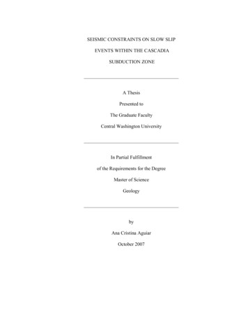
CHAPTER IINTRODUCTIONThe Cascadia subduction zone of the northwestern United States andsouthwestern Canada is a 1000-km thrust fault that stretches from northern California toVancouver Island. Here, the Juan de Fuca plate is subducted beneath the North Americaplate. This interface is thought to be seismically active, in that magnitude Mw 9 thrustearthquakes have ruptured the shallow interface repeatedly every several hundred years(Atwater et al., 1987; Satake et al., 1996; Atwater et al., 1997). There is geological andhistorical evidence that suggests that the last one of these large events occurred in 1700as a Mw 9 earthquake (Satake et al., 1996; Satake et al., 2003; Atwater et al., 2005).About 5 years ago it was determined that another process occurs in this subduction zoneand in other subduction zones of the world.It has been recognized that a large portion of the deeper Cascadia subduction zoneis aseismically slipping, down-dip of the locked zone, at around 25 km to 45 km depth(Figure 1). Evidence for this was provided by continuous geodetic measurements fromseven global positioning system (GPS) sites that measured a transient reversal from thelong term northeastward motion into an extension SE-directed motion. (Dragert et al.,2001). This process was also observed with GPS in other places of the world after a fewlarge subduction earthquakes. During the weeks after these events; such as the 1995 Mw 8.0 Jalisco (Mexico) event, the 1994 Mw 7.7 Sanriku (Japan) event, and the 2001 Mw 8.4 Peru event, there was postseismic motion with additional moment release (Melbourneet al., 2002).1
2Figure 1. Depth contours of the Cascadia subduction zone. The subduction zone starts innorthern California and ends at Vancouver Island. The black numbers represent the depthon each of the contours (red).It was first thought that this type of event released large amounts of strain energywithout any detectable seismic shaking (Linde et al., 1988), but it was later recognizedthat a subtle seismic signature does accompany this slow creep. The slip events wereassumed to have rupture rates lower than those that can be detected by most forms ofseismic instrumentation (Melbourne et al., 2002) and it was not possible to see this signalbefore. As mentioned before, slow slip events (SSE) like these have now been found inmany convergent margins other than Cascadia such as Mexico, Alaska, Japan and CostaRica, lasting from a few days to as long as a few years (Ozawa et al., 2002).
3In the case of Cascadia, initial studies showed that these events have been takingplace every 14.5 1 months for the past 10 years (Miller et al., 2002). More recentstudies demonstrate that the periodicity varies within the different areas that form theCascadia subduction zone: there is a periodicity of 10.9 1.2 months under northernCalifornia and an 18 2 month periodicity offshore central Oregon (Szeliga et al., 2004).This regular and cyclical nature of the transient events indicates that they are afundamental mode of strain release in subduction zones, and they may contribute to thestrain build-up that can result in a great earthquake.The first seismic signals related to the slow slip events were originally noticed inthe Japan fore arc region, where the Philippine Sea plate is subducting under the Eurasianplate. Using a borehole seismograph network, Japanese scientists were able to find tremorbursts that lasted a few minutes to a few days (Obara, 2002). Afterward, in Cascadiathese non-volcanic tremors were recognized using the regional surface seismic network.These are pulsating, deep tremor-like seismic signals (Rogers and Dragert, 2003) that areusually observed at active volcanic areas. Besides Japan and Cascadia, this type ofnonvolcanic tremor has also been detected in the San Andreas fault (Nadeau and Dolec,2005) and the Alaskan subduction zone (Peterson et al., 2005).Tremor location is difficult, primarily because they do not look like regularearthquake waves in a seismogram, with discernible P and S phases. Instead, tremor isvery clustered, emergent and noisy, and the onset time is extremely hard to pick,obfuscating depth constraints. Also, they have a high frequency content of 1 to 5 Hz(lower than regular earthquakes) which causes them to be sensitive to small-scale crustal
4structures, therefore making them even noisier signals by the time they reach the surfaceseismometers.The first approach to analyzing the nonvolcanic episodic tremor-and-slip (ETS) inCascadia assumed that tremor bursts were located near or along the subduction interface(Rogers and Dragert, 2003). But by using a source-scanning algorithm (Kao et al., 2005),which uses a brightness function on the grid points of the subduction zone to identify theexistence of seismic sources in time and space, it was determined that tremor bursts arewidely distributed over a 40-km depth range, and that they are bounded approximately bythe surface projections of 30- and 45-km depth contours of the subduction plate interface(Kao et al., 2005). When the seismic data are Band-pass filtered to 1–6 Hz and rectified,signals of the tremor prove to be strongest on the horizontal components. Using a onedimensional S-wave velocity model, hypocenters of tremor bursts were determined withdepth errors of 5 to 10 km. The results of this method were consistent with the last result,which were that tremors signals have an apparent velocity of 3.8–4.2 km/s and thattremor depths are distributed over a wide range (including the overriding crust and thesubducting slab) greater than the errors (McCausland et al., 2005). The observed depthrange implied that tremors could be associated with the variation of stress field inducedby the transient slip events.These tremor bursts have not been located directly on the plate interface, but thereis little doubt that they are related to the slow slip events. So it was necessary to explaintheir existence with another process related to the slip. The process that has beensuggested is the movement of fluids: dehydration of fluids on the plate interface to its
5surroundings traveling through cracks might cause these tremor bursts by changing thepressure in the system (Obara, 2002; Kao et al., 2005; McCausland et al., 2005).In 2006 it was discovered in the Nankai subduction zone that there are also othermechanisms releasing stress in the transition zone during these GPS-detectable events.These new signals where named low frequency earthquakes (LFE) because it is usuallyonly possible to identify their S-wave arrivals (Shelly et al., 2006). These events werelocated to the plate interface and have a shear slip mechanism. Cross-correlating LFEsuggested that low frequency tremor may be a superposition of these LFE (Shelly et al.,2006); in other words, that tremor bursts also originate from small thrust faults along theplate interface.After the LFE were found, another signal was identified between the tremorbursts in Japan. These where named very low frequency (VLF) earthquakes. They have avery long period of as much as 20 s and are indeed happening at the same time and alsohave a similar migration as the tremor bursts (Ito et al., 2006). The VLF earthquakes havea thrust mechanism and are bound to the plate interface at depths of 30–35 km (Ito et al.,2006). This result is important because it brings us one step closer to understanding themechanism triggering slow slip events.To further investigate the mechanism of the LFE, Ide et al. (2007) analyzed thefirst arrival P-wave and an inversion of the empirical moment tensor of the S-waveseparately. Both analyses yield the same result; that is, that LFE are a result of shear slipon a low angle fault (Ide et al., 2007), and they are consistent with the SSE thrustmechanisms shown in previous studies (Hirose and Obara, 2005). Finally, by using a
6match filter technique on the tremor bursts to see if they correlate with the LFE, it wasfound that during high tremor times the LFE sequences are almost continuous; so tremorsignals are now believed to be a swarm of LFE generated by many small shear slip eventson the plate interface (Shelly et al., 2007).Cascadia is one of the largest subduction zones on Earth, akin to the Sundamegathrust which produced the 2004 Sumatra (Mw 9.3, 300 000 deaths) great earthquake,and populated with 6–7 million people on the forearc. With the discovery of the SSE andETS with GPS, we now have a major new constraint on the Cascadia energy budget. GPSis limited by daily measurements, sparse coverage, and non-unique inversions. Tremor bycontrast, clearly gives moment-by-moment details of slip evolution so it can be used as ahigher resolution instrument to find out more about these SSE.If this model is correct, and given the noted difficulty in determining hypocentrallocations (particularly depth for tremor sources), it makes sense to ascertain whethertremor follows magnitude—frequency relationships inferred for other tectonic regimes.Since magnitudes cannot be assigned to tremor bursts until the source of the mechanismis better understood, it makes sense to instead attempt to quantify the frequency—duration aspects of tremor, whether it varies over time, and in particular whether it variesduring the largest, GPS-detectable slow slip events.The importance of doing further investigation on this topic is that there arereasons to think that big megathrust events will be triggered by SSE, which, as mentionedbefore, are not only recognized in Cascadia but also in other faults such as the SanAndreas fault (Nadeau and Dolec, 2005), and are likely ubiquitous in all active faults.
7Furthermore, these SSE are dissipating energy at the lower end of the locked zone, sothey delineate the seismic hazard to cities, such as Seattle, that lie near the top of theforearc of large subduction zones. Finally, to asses this seismic hazard it is also necessaryto know by what amount they are reducing the strain that might be released by the largesubduction zone earthquakes.The specific aspects of tremor addressed here are as follows:1. Does tremor follow anything resembling known frequency—magnituderelationships? Is it a log–linear relationship and what are the b-values?2. If not, then what does a typical distribution look like?3. Does the frequency—duration relationship change during the largest slowearthquakes?4. What percentage of total tremor time is released during an SSE versus all the othertime?5. Does average tremor amplitude increase during GPS events, or is it only the durationthat varies during this time?6. Where are tremor sources located during the January 2007 event?7. Does tremor coincide with the down dip limit of transient slip as inferred from GPSinversions?These questions were addressed under the assumption that GPS-observeddeformation transients and tremor bursts are different manifestations of the same sheardislocation process at depth.
CHAPTER IIDATA PROCESSINGThere are various seismic networks across the Pacific Northwest: the PacificNorthwest Seismographic Network (PNSN), a surface network run by the United StatesGeological Survey and the University of Washington that monitors seismicity in thestates of Washington and Oregon; the Plate Boundary Observatory (PBO) boreholenetwork, which is part of the EarthScope project run by UNAVCO, Inc.; theTransportable Array (TA), which is part of the Incorporated Research Institutions forSeismology (IRIS) and EarthScope USArray; and the EarthScope funded CascadiaArrays For EarthScope (CAFE) experiment network. Seismic data from these fourdifferent networks were obtained from the IRIS Data Management Center (DMC) Website covering the time span from July of 2005 to February of 2007 (Figure 2). This timeperiod was selected mainly because it contains two of the latest GPS-detectable eventswhich are the September 2005 event and the January 2007 event.The data, after they had been requested, were delivered via file transfer protocol(ftp) in SEED format. The seed files were converted to a format suitable for use in theSeismic Analysis Code (SAC) program. This program is a tool used to make detailedanalysis of any kind of seismic data.Merging the DataThe data, as stored by IRIS comes in many separate pieces, including parts of aday or even parts of two different days together. The first step was to merge all the8
9Figure 2. Map of stations from the four seismic networks used. The different colorsrepresent the different networks. Red represents the Pacific Northwest SeismographicNetwork stations, yellow represents the Plate Boundary Observatory stations, greenrepresents the Transportable Array stations and blue represents the Cascadia Array ForEarthScope stations. Modified from Google Earth.pieces of data into daily files so the data could be analyzed one day at a time and differentstations could be compared using a single metric. To do this it was necessary to first cutfiles with parts of two different days in them, and this was accomplished using theprogram called chop day.pl. This program would take each sac file, open it using SAC,cut the parts of different days and rename the new cut files using the respective date andtime. After running chop day.pl on all the files, the seismic data were ready to bemerged. A new program was written for this, dailify.pl, and it uses SAC to read all the
10sac files for one day and merge them together into one file containing a complete day ofdata (Figure 3). The files created by this program where named with the formatYYYY.DOY.STA.COMP.sac; as an example the file 2006.204.CPW.EHZ.sac would bethe file corresponding to the year 2006, day of year 204, station CPW, and componentEHZ.Figure 3. Example of merged data. The merging process was done for six differentstations on September 10 of 2005. This data shows various tremor bursts across the day.This is for day 253 of 2005.Data ReductionEvery daily file is around 30 Mb in size, so to be able to work with years of datain a time efficient way, it is necessary to bring this number down. Before the size can bereduced, the first step is to remove the velocity sensitivity or gain of each station. Stationgains vary as a consequence of the different types of stations: broadband, short-period,
11etc. By doing this, all the stations can be compared on the same scale, which is requiredto obtain the averages of the seismic files for one day. To do this, the program degain.plreads in a seismic file containing one day of data and gets the gain information for eachstation and each component from a text file containing the velocity sensitivity in countsper meter per second. Using a SAC module, the gain is removed from each of the dailyfiles dividing each data point by the gain corresponding to that station and component.Then it outputs a new file containing the degained data.Now, to finally reduce the size of the daily files, it is necessary to decimate thedata. The raw data contains files that are 100 samples per second (sps), and by using theprogram decimate.pl (created for this same purpose), which also uses a SAC module, theseismic files are decimated to 10 sps each. These new files are around 3.2 to 3.4 Mb each,which is significantly smaller than the raw data ( 30 Mb).Data SelectionNow that the size of the seismic files has been reduced, a data selection has to bedone. In order to average the files, it is necessary that all files that are to be merged for aparticular day have the same number of points. The files that contain data for less than 23hours of one day are discarded, and the remaining files are cut to the number of points ofthe smallest file remaining (longer than 23 hours) for that same day of the year. Thisselection and cutting processes are done using the Perl program called cut.pl that uses aSAC module to do all this. The remaining files that have been cut have to go throughanother selection. It is necessary to make sure that these files all start at 00:00:00 hours ofthe day. If they don’t, they are dropped because by the time the files are averaged, they
12would be shifted to the right giving a wrong average. This final selection process is donewith final cut.pl also using a SAC module.Calculating the AveragesThe averages of each day of the seismic data are done using the envelope functionof the files. After selecting the data to be used in the analysis, the envelopes of the filescan be calculated. These are essential for automatically quantifying tremor burst, becausethey give a positive scale of the seismic trace. The Perl program envelope.pl was createdfor this purpose. This program opens the file in SAC, squares it, applies the square root,and then calculates the envelope function using a Hilbert transform. This program outputsa new file for each seismic file containing its envelope function (Figure 4a).The averages are calculated for each day of the year. Using the programaverage.pl, the files for one day of the year and different regionally adjacent stations aresummed up and then divided by the number of files summed to get the average of thatday (Figure 4b).SummaryHere I present a summary of Perl codes written to process the data in the orderthey had to be run, their names, and their purpose (Table 1). This may serve as a tool forfurther use of the programs outside of this thesis.
13Figure 4. Example of envelope functions. (a) Envelope functions of the seismic data from5 different stations that survived the data processing for day 253 of 2005. Each of thespikes across the data represents a tremor burst that might be composed of more bursts.(b) Average of those same five envelope functions.
14Table 1Summary of Programs Written for Data ProcessingProgram NameFunctionchop day.plSeparates files that contain data for different days of the year andcreates new files with the separated pieces of data.dailify.plGets the chopped files (output of chop day.pl) and merges them intodaily files.degain.plRemoves the gain of all the different stations of which the seismicdata come from.decimate.plTurns the degained files (output of degain.pl), which are 100 sps files,into 10 sps filescut.plEliminates daily files shorter than 23 hours, and then cuts theremaining files to the number of points of the shortest file in the list,so they all have the same number of points.final cut.plFrom the remaining files (output of cut.pl), it eliminates the ones thatdo not start at the beginning of the day (time 00:00:00).envelope.plUses the output of final cut.pl and calculates the envelope function ofthem.average.plTakes all the envelope files (output of envelope.pl) and calculates anaverage of these files for each day of the year separately.
CHAPTER IIITREMOR QUANTIFICATIONOnce the regional averages are computed, it is assumed that any signal thatsurvives the envelope stacks is tectonic in origin, given that local ground noise should notstack coherently. For each regional averaged file, tremor is identified and summed in thefollowing manner: all times in which the regional envelope average exceeds a thresholdvalue of the velocity amplitude is considered to be active tremor; less than this value isconsidered noise. Picking the threshold is a difficult task and it is done manually,typically using a day where tremor bursts are obvious (Figure 5).Figure 5. Example of the data average for day 253 of 2005. (a) Average of all theenvelope functions of the stations that survived the data processing and cutting on day253 of the year 2005. (b) Area of that day showing in detail how threshold value (reddashed line) is picked using a high tremor day.15
16Using this method, tremor was counted for all the collected data, which goes fromJune of 2005 to February of 2007. The threshold value varied a lot during this period,being lower during times of high tremor and GPS detectable events; and higher duringtimes of no detectable events. Even though there are no tremor bursts correlating acrossstations during the times of no detectable events, the noise signal is predominant in thesetimes and as different stations are averaged the noise amplitudes get enlarged. Asmentioned before, this time period contains two of the latest SSE which are theSeptember 2005 event and the January 2007 event (Figure 6).Taking into account all 19 months of data, 627.5 hours of tremor were countedof which 284.95 hours come from the September 2005 event and 238.38 hours belong tothe January 2007 event. It is very clear on Figure 6 where the two GPS-detectable eventsare. The results show that around 80% of the total energy released during the 19 monthsis released during the big events, but 20% of the energy was released during other times,when there are no detectable GPS events.Moment Magnitude—Tremor Time RelationshipIt is now known how many hours of tremor occurred during both the 2005 and2007 events which correlate well with results from different research groups(McCausland et al., 2005) which have also counted the hours of tremor for additionalprevious events starting in 2003 (McCausland et al., 2005). These results are shown inTable 2.Each of these events has already been assigned a slip distribution calculated fromGPS (Szeliga et al., 2007), which where used to calculate the inferred moment magnitude
04/23
Central Washington University In Partial Fulfillment of the Requirements for the Degree Master of Science Geology by Ana Cristina Aguiar October 2007 . ii CENTRAL WASHINGTON UNIVERSITY Graduate Studies We hereby approve the thesis of Ana Cristina Aguiar Candidate for the degree of Master of Science . Summary of Programs Written for Data .