Transcription
Talk V:Stochastic Properties and Multifractal AnalysisCincinnati (2009)Volker MAYERUniversité de Lille IU.M.R. CNRS 8524http://math.univ-lille1.fr/ mayer/joint work with Mariusz UrbańskiVolker MAYER (USTL)Stochastic Properties and MFA1 / 16
Introduction: Zdunik’s smooth or fractal theoremConsider pc (z) z 2 c and the associated Julia set Jc .Jc is connected iff c M the Mandelbrot set.Volker MAYER (USTL)Stochastic Properties and MFA2 / 16
Introduction: Zdunik’s smooth or fractal theoremConsider pc (z) z 2 c and the associated Julia set Jc .Jc is connected iff c M the Mandelbrot set.There are several dynamically important measures for the dynamical system (pc , Jc ).Volker MAYER (USTL)Stochastic Properties and MFA2 / 16
Introduction: Zdunik’s smooth or fractal theoremConsider pc (z) z 2 c and the associated Julia set Jc .Jc is connected iff c M the Mandelbrot set.There are several dynamically important measures for the dynamical system (pc , Jc ).A. Zdunik (in her 1990 Inv. Math paper) comparedthe Hausdorff measure HM δcwith the harmonic measure µc(in fact the measure of maximal entropy).Volker MAYER (USTL)Stochastic Properties and MFA2 / 16
Introduction: Zdunik’s smooth or fractal theoremConsider pc (z) z 2 c and the associated Julia set Jc .Jc is connected iff c M the Mandelbrot set.There are several dynamically important measures for the dynamical system (pc , Jc ).A. Zdunik (in her 1990 Inv. Math paper) comparedthe Hausdorff measure HM δcwith the harmonic measure µc(in fact the measure of maximal entropy).Theorem (Zdunik(Version for polynomials))δc Hdim(µc ) excepted if pc is a power map z 7 z d or a Chebychev polynomial.Volker MAYER (USTL)Stochastic Properties and MFA2 / 16
Introduction: Zdunik’s smooth or fractal theoremConsider pc (z) z 2 c and the associated Julia set Jc .Jc is connected iff c M the Mandelbrot set.There are several dynamically important measures for the dynamical system (pc , Jc ).A. Zdunik (in her 1990 Inv. Math paper) comparedthe Hausdorff measure HM δcwith the harmonic measure µc(in fact the measure of maximal entropy).Theorem (Zdunik(Version for polynomials))δc Hdim(µc ) excepted if pc is a power map z 7 z d or a Chebychev polynomial.Theorem (Makarov)If Jc is connected (hence A simply connected) then Hdim(µc ) 1.Volker MAYER (USTL)Stochastic Properties and MFA2 / 16
Introduction: Zdunik’s smooth or fractal theoremVolker MAYER (USTL)Stochastic Properties and MFA3 / 16
Introduction: Zdunik’s smooth or fractal theoremVolker MAYER (USTL)Stochastic Properties and MFA4 / 16
Introduction: Zdunik’s smooth or fractal theoremVolker MAYER (USTL)Stochastic Properties and MFA5 / 16
Introduction: Zdunik’s smooth or fractal theoremReason for the dichotomy in Zdunik’s result:Her work is based on stochastic limit theorems (Central Limit Theorem, Law of theIterated Logarithm) andVolker MAYER (USTL)Stochastic Properties and MFA6 / 16
Introduction: Zdunik’s smooth or fractal theoremReason for the dichotomy in Zdunik’s result:Her work is based on stochastic limit theorems (Central Limit Theorem, Law of theIterated Logarithm) andsmooth cases asymptotic variance σ 2 0.Volker MAYER (USTL)Stochastic Properties and MFA6 / 16
The action of Lt on Hölder spacesSetting.f : C Ĉ hyperbolic meromorphic of finite order s.t. f ′ (z) z α1 f (z) α2 .γ f (z) dz ′′Derivative wrt dσ γ dz z α2 : f (z) σ : f (z) γ(z) .Volker MAYER (USTL)Stochastic Properties and MFA7 / 16
The action of Lt on Hölder spacesSetting.f : C Ĉ hyperbolic meromorphic of finite order s.t. f ′ (z) z α1 f (z) α2 .γ f (z) dz ′′Derivative wrt dσ γ dz z α2 : f (z) σ : f (z) γ(z) .The transfer operator associated to the potential φt t log f ′ σ is given byXXLt g (w ) g (z)e φt g (z) f ′ (z) tσ .f (z) wVolker MAYER (USTL)(1)f (z) wStochastic Properties and MFA7 / 16
The action of Lt on Hölder spacesSetting.f : C Ĉ hyperbolic meromorphic of finite order s.t. f ′ (z) z α1 f (z) α2 .γ f (z) dz ′′Derivative wrt dσ γ dz z α2 : f (z) σ : f (z) γ(z) .The transfer operator associated to the potential φt t log f ′ σ is given byXXLt g (w ) g (z)e φt g (z) f ′ (z) tσ .f (z) w(1)f (z) wRecall that1 L̃t e P(t) Lt is the normalized operatorVolker MAYER (USTL)Stochastic Properties and MFA7 / 16
The action of Lt on Hölder spacesSetting.f : C Ĉ hyperbolic meromorphic of finite order s.t. f ′ (z) z α1 f (z) α2 .γ f (z) dz ′′Derivative wrt dσ γ dz z α2 : f (z) σ : f (z) γ(z) .The transfer operator associated to the potential φt t log f ′ σ is given byXXLt g (w ) g (z)e φt g (z) f ′ (z) tσ .f (z) w(1)f (z) wRecall that1 L̃t e P(t) Lt is the normalized operator2 L̃t fixes the density ρt dµt /dmt (hence 1 is eigenvalue).Volker MAYER (USTL)Stochastic Properties and MFA7 / 16
The action of Lt on Hölder spacesSetting.f : C Ĉ hyperbolic meromorphic of finite order s.t. f ′ (z) z α1 f (z) α2 .γ f (z) dz ′′Derivative wrt dσ γ dz z α2 : f (z) σ : f (z) γ(z) .The transfer operator associated to the potential φt t log f ′ σ is given byXXLt g (w ) g (z)e φt g (z) f ′ (z) tσ .f (z) w(1)f (z) wRecall that1 L̃t e P(t) Lt is the normalized operator2 L̃t fixes the density ρt dµt /dmt (hence 1 is eigenvalue).Now we have to1 let Lt act on Hölder functions. Given h : J C, letf h(y ) h(x) vβ (h) supforallx,y Jwith0 y x δ,f y x βbe the β-variation of the function h. Consider the space of β-Hölder or simplyHölder continuous functionsHβ (Jf ) {h : Jf C : h β }Volker MAYER (USTL)with normStochastic Properties and MFA h β vβ (h) h .7 / 16
The action of Lt on Hölder spacesSetting.f : C Ĉ hyperbolic meromorphic of finite order s.t. f ′ (z) z α1 f (z) α2 .γ f (z) dz ′′Derivative wrt dσ γ dz z α2 : f (z) σ : f (z) γ(z) .The transfer operator associated to the potential φt t log f ′ σ is given byXXLt g (w ) g (z)e φt g (z) f ′ (z) tσ .f (z) w(1)f (z) wRecall that1 L̃t e P(t) Lt is the normalized operator2 L̃t fixes the density ρt dµt /dmt (hence 1 is eigenvalue).Now we have to1 let Lt act on Hölder functions. Given h : J C, letf h(y ) h(x) vβ (h) supforallx,y Jwith0 y x δ,f y x βbe the β-variation of the function h. Consider the space of β-Hölder or simplyHölder continuous functionsHβ (Jf ) {h : Jf C : h β }2with norm h β vβ (h) h .Potential of the form φ t log f ′ σ h, h Hβ (Jf ).Denote associated normalized operator by L̃φ .Volker MAYER (USTL)Stochastic Properties and MFA7 / 16
The action of Lt on Hölder spacesTwo Norm inequality and Spectral GapThe key ingredient for all what follows is the two norm inequality:LemmaIf φ t log f ′ σ h, h Hβ (Jf ) then there exists a constant c1 0 such that L̃nφ g β 1 g β c1 g 2for all n 1 large enough and every g Hβ . In particular, L̃φ (Hβ ) Hβ .Volker MAYER (USTL)Stochastic Properties and MFA8 / 16
The action of Lt on Hölder spacesTwo Norm inequality and Spectral GapThe key ingredient for all what follows is the two norm inequality:LemmaIf φ t log f ′ σ h, h Hβ (Jf ) then there exists a constant c1 0 such that L̃nφ g β 1 g β c1 g 2for all n 1 large enough and every g Hβ . In particular, L̃φ (Hβ ) Hβ .Modulo some details,this allows to apply Ionescu-Tulcea and Marinescu in order to get:Theorem- Spectral Gap: The number 1 is a simple isolated eigenvalue of L̃φ : Hβ Hβ andthe rest of the spectrum is contained in D(0, r ) for some 0 r 1.- Decomposition: We have the decomposition L̃φ Q1 S where QR1 : Hβ Cρφ isa projector on the eigenspace Cρφ (given by the formula Q1 (g ) ( g dmφ )ρφ ),Q1 S S Q1 0 and S n β C ξ nfor some constant C 0, some constant ξ (0, 1) and all n 1.Volker MAYER (USTL)Stochastic Properties and MFA8 / 16
The action of Lt on Hölder spacesTheorem- Spectral Gap: The number 1 is a simple isolated eigenvalue of L̃φ : Hβ Hβ andthe rest of the spectrum is contained in D(0, r ) for some 0 r 1.- Decomposition: We have the decomposition L̃φ Q1 S where QR1 : Hβ Cρφ isa projector on the eigenspace Cρφ (given by the formula Q1 (g ) ( g dmφ )ρφ ),Q1 S S Q1 0 and S n β C ξ nfor some constant C 0, some constant ξ (0, 1) and all n 1.RemarkL̃φ : Cb (Jf ) Cb (Jf ) does not have a spectral gap!Volker MAYER (USTL)Stochastic Properties and MFA9 / 16
The action of Lt on Hölder spacesTheorem- Spectral Gap: The number 1 is a simple isolated eigenvalue of L̃φ : Hβ Hβ andthe rest of the spectrum is contained in D(0, r ) for some 0 r 1.- Decomposition: We have the decomposition L̃φ Q1 S where QR1 : Hβ Cρφ isa projector on the eigenspace Cρφ (given by the formula Q1 (g ) ( g dmφ )ρφ ),Q1 S S Q1 0 and S n β C ξ nfor some constant C 0, some constant ξ (0, 1) and all n 1.RemarkL̃φ : Cb (Jf ) Cb (Jf ) does not have a spectral gap!Corollary (Mixing)With the previous notations we have, for every n 1, that L̃nφ Q1 S n and that Z L̃nφ (g ) g dmφ ρφ kS n (g )kβ C ξ n kg kβ , g Hβ .βHence,L̃nφ (g ) RVolker MAYER (USTL) g dmφ ρφ exponentially when n .Stochastic Properties and MFA9 / 16
Stochastic properties: Decay of correlations and CLTThis topic concerns the asymptotic behavior of Sn ψ Pn 1n 0ψ f k for appropriate ψ.Since the equilibrium state µφ is ergodic it follows from Birkhoffs Ergodic Theorem thatZ1Sn ψ(z) ψ dµφ for µφ a.e. z Jf .nRIn the centered case ( ψ dµφ 0), that we consider from now on, n1 Sn ψ 0 µφ –a.e.The random variables Xk ψ f k have same distribution (µφ is invariant).Volker MAYER (USTL)Stochastic Properties and MFA10 / 16
Stochastic properties: Decay of correlations and CLTThis topic concerns the asymptotic behavior of Sn ψ Pn 1n 0ψ f k for appropriate ψ.Since the equilibrium state µφ is ergodic it follows from Birkhoffs Ergodic Theorem thatZ1Sn ψ(z) ψ dµφ for µφ a.e. z Jf .nRIn the centered case ( ψ dµφ 0), that we consider from now on, n1 Sn ψ 0 µφ –a.e.The random variables Xk ψ f k have same distribution (µφ is invariant).The classical Central Limit Theorem (CLT) says that 1n Sn ψ converges in distribution toa Gaussian random variable N (0, σ 2 ) if σ 2 0 and if the variables Xk are independent.Volker MAYER (USTL)Stochastic Properties and MFA10 / 16
Stochastic properties: Decay of correlations and CLTThis topic concerns the asymptotic behavior of Sn ψ Pn 1n 0ψ f k for appropriate ψ.Since the equilibrium state µφ is ergodic it follows from Birkhoffs Ergodic Theorem thatZ1Sn ψ(z) ψ dµφ for µφ a.e. z Jf .nRIn the centered case ( ψ dµφ 0), that we consider from now on, n1 Sn ψ 0 µφ –a.e.The random variables Xk ψ f k have same distribution (µφ is invariant).The classical Central Limit Theorem (CLT) says that 1n Sn ψ converges in distribution toa Gaussian random variable N (0, σ 2 ) if σ 2 0 and if the variables Xk are independent.The later is however not the case and the defect of independence of ψ and U n ψ ψ f nis measured by the correlationsRRRCn (ψ1 , ψ2 ) : ψ1 · (ψ2 f n ) dµφ ψ1 dµφ ψ2 dµφ R (ψ1 E ψ1 ) (ψ2 E ψ2 ) f n dµφ ,Rwhere we put E ψ ψ dµφ .RIn the centered case E ψ1 E ψ2 0, then Cn (ψ1 , ψ2 ) ψ1 ψ2 f n dµφ .Volker MAYER (USTL)Stochastic Properties and MFA10 / 16
Stochastic properties: Decay of correlations and CLTDecay of CorrelationsTheoremFor all (centered) ψ1 Oβ”mainly Hölder”,ψ2 L1 (mφ ) Cn (ψ1 , ψ2 ) ξ n kL̃φ (ψ1 ρφ )kβ kψ2 kL1 (mφ ) ,where ξ (0, 1) comes from the spectral gap Theorem.Volker MAYER (USTL)Stochastic Properties and MFA11 / 16
Stochastic properties: Decay of correlations and CLTDecay of CorrelationsTheoremFor all (centered) ψ1 Oβ”mainly Hölder”,ψ2 L1 (mφ ) Cn (ψ1 , ψ2 ) ξ n kL̃φ (ψ1 ρφ )kβ kψ2 kL1 (mφ ) ,where ξ (0, 1) comes from the spectral gap Theorem.Proof.Remember that µφ ρφ mφ . Therefore,ZZCn (ψ1 , ψ2 ) ψ1 ψ2 f n ρφ dmφ L̃nφ (ψ1 ρφ )ψ2 dmφ .But L̃nφ (ψ1 ρφ ) S n 1 (L̃φ (ψ1 ρφ )) cξ n 1 kL̃φ (ψ1 ρφ )kβ(2)because of the Corollary ”Mixing” and since L̃φ (ψ1 ρφ ) Hβ . Hence, Cn (ψ1 , ψ2 ) ξ n kL̃φ (ψ1 ρφ )kβ kψ2 kL1 (mφ )as claimed.Volker MAYER (USTL)Stochastic Properties and MFA11 / 16
Stochastic properties: Decay of correlations and CLTCentral limit TheoremFrom decay of correlations we can get CLT via Liverani-Gordin’s method.PkLet us recall that CLT means that 1n Sn ψ 1n n 1k 0 U ψ(z) converges in distribution2to the Gaussian random variable N (0, σ ). More precisely, for any t R, Z t11 µ {z Jf :Sn ψ(z) t} exp[ u 2 /2σ 2 ] du.nσ 2π Volker MAYER (USTL)Stochastic Properties and MFA12 / 16
Stochastic properties: Decay of correlations and CLTCentral limit TheoremFrom decay of correlations we can get CLT via Liverani-Gordin’s method.PkLet us recall that CLT means that 1n Sn ψ 1n n 1k 0 U ψ(z) converges in distribution2to the Gaussian random variable N (0, σ ). More precisely, for any t R, Z t11 µ {z Jf :Sn ψ(z) t} exp[ u 2 /2σ 2 ] du.nσ 2π Theorem′If ψ S t log f σ h, t R and h a Hölder function, or, more generally, ifψ β (0,1] Oβ , then the asymptotic variance2σ σµ2 φ (ψ) σ̂µ2 φ (ψ) Z2ψ dµφ 2 ZXk 1ψ ψ f k dµφ(3)exists and one of the following two cases occurs:(i) If σ 2 0, then the CLT holds.(ii) If σ 2 0, then Uψ ψ f is measurably cohomologous to zero.In addition, if ψ is a bounded function, then equality in (3) holds.Volker MAYER (USTL)Stochastic Properties and MFA12 / 16
Multifractal Analysis of Gibbs statesMultifractal analysisThe following notions are valid for any measures but we focus on the conformal measuresmφ and the equilibrium states µφ . The pointwise dimension of µφ at z Jf is given bydµφ (z) limr 0log µφ (D(z, r ))log r(4)provided this limit exists. Note that dµφ (z) dmφ (z) since dµφ ρφ dmφ .Volker MAYER (USTL)Stochastic Properties and MFA13 / 16
Multifractal Analysis of Gibbs statesMultifractal analysisThe following notions are valid for any measures but we focus on the conformal measuresmφ and the equilibrium states µφ . The pointwise dimension of µφ at z Jf is given bydµφ (z) limr 0log µφ (D(z, r ))log r(4)provided this limit exists. Note that dµφ (z) dmφ (z) since dµφ ρφ dmφ .The object of the multifractal formalism is the geometric study of the level sets Dφ (α) z Jr (f ) ; dµφ (z) α .Volker MAYER (USTL)Stochastic Properties and MFA(5)13 / 16
Multifractal Analysis of Gibbs statesMultifractal analysisThe following notions are valid for any measures but we focus on the conformal measuresmφ and the equilibrium states µφ . The pointwise dimension of µφ at z Jf is given bydµφ (z) limr 0log µφ (D(z, r ))log r(4)provided this limit exists. Note that dµφ (z) dmφ (z) since dµφ ρφ dmφ .The object of the multifractal formalism is the geometric study of the level sets Dφ (α) z Jr (f ) ; dµφ (z) α .(5)and of the fractal spectrumFφ (α) Hdim(Dφ (α))Volker MAYER (USTL)Stochastic Properties and MFA(6)13 / 16
Multifractal Analysis of Gibbs statesMultifractal analysisThe following notions are valid for any measures but we focus on the conformal measuresmφ and the equilibrium states µφ . The pointwise dimension of µφ at z Jf is given bydµφ (z) limr 0log µφ (D(z, r ))log r(4)provided this limit exists. Note that dµφ (z) dmφ (z) since dµφ ρφ dmφ .The object of the multifractal formalism is the geometric study of the level sets Dφ (α) z Jr (f ) ; dµφ (z) α .(5)and of the fractal spectrumFφ (α) Hdim(Dφ (α))(6)Strategy: Show that Fφ (α) is Legendre conjugate to the Temperature T (q).One associates somehow to the set Fφ (α) a pair of auxiliary measures µq , mq (q q(α))which detect the dimension of fdim(α)exactly like ”mh ” gives the dimension of Λc in Bowen’s Formula.Volker MAYER (USTL)Stochastic Properties and MFA13 / 16
Multifractal Analysis of Gibbs statesTemperature functionAssumption: f : C Ĉ hyperbolic, dynamically regular and of divergence type, hencewhich allows to define the temperature function: letϕ t log f ′ σ h, h bounded Hölder.May suppose ϕ is normalized, i.e. P(ϕ) 0 (otherwise take ϕ P(ϕ)).Volker MAYER (USTL)Stochastic Properties and MFA14 / 16
Multifractal Analysis of Gibbs statesTemperature functionAssumption: f : C Ĉ hyperbolic, dynamically regular and of divergence type, hencewhich allows to define the temperature function: letϕ t log f ′ σ h, h bounded Hölder.May suppose ϕ is normalized, i.e. P(ϕ) 0 (otherwise take ϕ P(ϕ)).SetVolker MAYER (USTL)ϕq,T qϕ T log f ′ σ, q R and T θ qt.Stochastic Properties and MFA14 / 16
Multifractal Analysis of Gibbs statesTemperature functionAssumption: f : C Ĉ hyperbolic, dynamically regular and of divergence type, hencewhich allows to define the temperature function: letϕ t log f ′ σ h, h bounded Hölder.May suppose ϕ is normalized, i.e. P(ϕ) 0 (otherwise take ϕ P(ϕ)).Setϕq,T qϕ T log f ′ σ, q R and T θ qt.Lemma-DefinitionFor every q R there exists a unique T T (q) θ qt such that P(ϕq,T ) 0.q 7 T (q) is called the temperature.Volker MAYER (USTL)Stochastic Properties and MFA14 / 16
Multifractal Analysis of Gibbs statesCase q 0: Then φ0,T T log f ′ σ and T (q 0) h the only zero ofT 7 P( T log f ′ σ ).Bowen’s Formula: T (0) h HD(Jr (f )).Volker MAYER (USTL)Stochastic Properties and MFA15 / 16
Multifractal Analysis of Gibbs statesCase q 0: Then φ0,T T log f ′ σ and T (q 0) h the only zero ofT 7 P( T log f ′ σ ).Bowen’s Formula: T (0) h HD(Jr (f )). We will see that for µ h log f ′ σ , m T log f ′ σthe domain of the multifractal spectrum Fφ is the singleton α h and then Fφ (h) h.Volker MAYER (USTL)Stochastic Properties and MFA15 / 16
Multifractal Analysis of Gibbs statesCase q 0: Then φ0,T T log f ′ σ and T (q 0) h the only zero ofT 7 P( T log f ′ σ ).Bowen’s Formula: T (0) h HD(Jr (f )). We will see that for µ h log f ′ σ , m T log f ′ σthe domain of the multifractal spectrum Fφ is the singleton α h and then Fφ (h) h.Main facts about the temperature:TheoremThe temperature function q 7 T (q) is real analytic with T ′ (q) 0 and T ′′ (q) 0. Inaddition the following are equivalent:1T ′′ vanishes in one point.2T ′′ vanishes at all points.34µφ µT ′ (q) log f ′ τ .φ and T ′ (q) log f ′ τ are cohomologous modulo a constant in the class of all Höldercontinuous functions.If one of these properties holds then T ′ (q) is constant equal to the only zero of thepressure function t 7 P( t log f ′ τ ) which is h HD(Jr (f )).Volker MAYER (USTL)Stochastic Properties and MFA15 / 16
Multifractal Analysis of Gibbs statesThe culminating result on MFA is:TheoremLet f : C Ĉ be a divergence type and dynamically regular meromorphic function oforder ρ 0 and let ϕ t log f ′ τ h be a tame potential. Then the followingstatements are true.1For every q R,Fφ (α) αq T (q)with α T ′ (q).If µφ 6 µ h log f ′ τ then the functions α 7 Fφ ( α) and T (q) form a Legendretransform pair.Volker MAYER (USTL)Stochastic Properties and MFA16 / 16
Multifractal Analysis of Gibbs statesThe culminating result on MFA is:TheoremLet f : C Ĉ be a divergence type and dynamically regular meromorphic function oforder ρ 0 and let ϕ t log f ′ τ h be a tame potential. Then the followingstatements are true.1For every q R,Fφ (α) αq T (q)with α T ′ (q).If µφ 6 µ h log f ′ τ then the functions α 7 Fφ ( α) and T (q) form a Legendretransform pair.2The function α 7 Fφ (α) is real-analytic throughout its whole domain(α1 , α2 ) [0, ).Volker MAYER (USTL)Stochastic Properties and MFA16 / 16
Multifractal Analysis of Gibbs statesThe culminating result on MFA is:TheoremLet f : C Ĉ be a divergence type and dynamically regular meromorphic function oforder ρ 0 and let ϕ t log f ′ τ h be a tame potential. Then the followingstatements are true.1For every q R,Fφ (α) αq T (q)with α T ′ (q).If µφ 6 µ h log f ′ τ then the functions α 7 Fφ ( α) and T (q) form a Legendretransform pair.23The function α 7 Fφ (α) is real-analytic throughout its whole domain(α1 , α2 ) [0, ).α1 α2 if and only if µφ µ h log f ′ τ with h HD(Jr (f )) (and thenα1 α2 h).Volker MAYER (USTL)Stochastic Properties and MFA16 / 16
Multifractal Analysis of Gibbs statesThe culminating result on MFA is:TheoremLet f : C Ĉ be a divergence type and dynamically regular meromorphic function oforder ρ 0 and let ϕ t log f ′ τ h be a tame potential. Then the followingstatements are true.1For every q R,Fφ (α) αq T (q)with α T ′ (q).If µφ 6 µ h log f ′ τ then the functions α 7 Fφ ( α) and T (q) form a Legendretransform pair.23The function α 7 Fφ (α) is real-analytic throughout its whole domain(α1 , α2 ) [0, ).α1 α2 if and only if µφ µ h log f ′ τ with h HD(Jr (f )) (and thenα1 α2 h).(we even have analyticity in the case of holomorphic families fλ ).Volker MAYER (USTL)Stochastic Properties and MFA16 / 16
Introduction: Zdunik's smooth or fractal theorem Consider p c(z) z2 c and the associated Julia set J c. J c is connected iff c Mthe Mandelbrot set. There are several dynamically important measures for the dynamical system (pc,J c). A. Zdunik (in her 1990 Inv. Math paper) compared the Hausdorff measure HMδc with the harmonic measure µ