WIXLIB

true both in-sample and out-of-sample.We also assess the importance of unspanned stochastic volatility when hedging an optionportfolio. Hedging the option portfolio solely with futures contracts causes only a small reduction in the variation in the portfolio profit-loss. However, consistent with the finding thatvolatility is largely unspanned by the futures contracts, adding one or two options to the set ofhedge instruments significantly reduces the variation in the portfolio profit-loss. Again, theseresults hold true both in-sample and out-of-sample as well as for different weighting schemesof the individual options in the portfolio.Our paper draws on the term structure literature. Using regression approaches similar tothe one applied in this paper, Collin-Dufresne and Goldstein (2002) and Heidari and Wu (2003)document the presence of unspanned stochastic volatility in the fixed income market. Theresults for the crude oil market are broadly consistent with the results reported in thesepapers.This appears to be the first stochastic volatility HJM-type model for pricing commodityderivatives.4 Previous HJM-type commodity models such as Cortazar and Schwartz (1994),Amin, Ng, and Pirrong (1995), Miltersen and Schwartz (1998), Clewlow and Strickland (1999)and Miltersen (2003) all assume deterministic volatilities.5 The advantage of working in anHJM setting is that unspanned stochastic volatility arises naturally.An alternative approach to pricing commodity derivatives relies on specifying the (typicallyaffine) dynamics of a limited set of state variables and deriving futures prices endogenously. Examples of this approach include Gibson and Schwartz (1990), Brennan (1991), Schwartz (1997),Hilliard and Reis (1998), Schwartz and Smith (2000), Richter and Sørensen (2002), Nielsenand Schwartz (2004) and Casassus and Collin-Dufresne (2005). Of these papers, only Richterand Sørensen (2002) and Nielsen and Schwartz (2004) explicitly allow for stochastic volatility.The main drawback of this modeling approach is that volatility is almost invariably completelyspanned by the futures contracts.64See Casassus, Collin-Dufresne, and Goldstein (2005) and Trolle and Schwartz (2008) for HJM-type modelsfor pricing interest rate derivatives.5Eydeland and Geman (1998) propose a stochastic volatility Heston (1993) model for pricing energy deriva-tives. However, they only model the evolution of the spot price, not the evolution of the entire futures curve.6Indeed, this is the case for the models in Richter and Sørensen (2002) and Nielsen and Schwartz (2004).Collin-Dufresne and Goldstein (2002) derive the parameter restrictions necessary for volatility to be unspannedin affine term structure models. Similar conditions can be derived for affine commodity models.4

The paper is organized as follows. Section 2 discusses the crude oil derivatives data thatwe make extensive use of throughout the paper. Section 3 presents model-free evidence ofunspanned stochastic volatility. Section 4 describes the model for pricing commodity derivatives in the presence of unspannned stochastic volatility. Section 5 discusses the estimationprocedure and estimation results. Section 6 concludes. Three appendices contain proofs andadditional information.2Overview of crude oil derivatives dataIn the paper we repeatedly use an extensive data set of crude oil futures and options tradingon the New York Mercantile Exchange (NYMEX). The NYMEX crude oil derivatives marketis the world’s largest and most liquid commodity derivatives market. The range of maturitiescovered by futures and options and the range of strike prices on the options are also greaterthan for other commodities. This makes it an ideal market for studying commodity derivativespricing. The raw data set consists of daily data from January 2, 1990 until May 18, 2006 onsettlement prices, open interest and daily volume for all available futures and options.7,8The number of futures and options and their maximum maturities have increased significantly through the sample period. From the first trading day in the sample to the last tradingday, the number of futures with positive open interest increased from 17 to 45 and the number of options with positive open interest increased from 77 to 1435. The maximum maturityamong futures with positive open interest increased from 499 to 2372 days, while the maximummaturity among options with positive open interest increased from 164 to 2008 days.9Liquidity has also increased significantly through the sample period. From the first tothe last trading day, open interest (daily volume) for the first futures contract with more7The NYMEX light, sweet crude oil futures contract trades in units of 1000 barrels. Prices are quoted asUS dollars and cents per barrel.8Note that all computations in the paper are based on settlement prices. Settlement prices for all contractsare determined by a “Settlement Price Committee” at the end of regular trading hours (currently 2.30 p.m.EST) and represent a very accurate measure of the true market prices at the time of close. Settlement pricesare widely scrutinized by all market participants since they are used for marking to market all account balances.9Futures contracts expire on the third business day prior to the 25th calendar day of the month precedingthe delivery month. If the 25th calendar day of the month is a non-business day, expiration is on the thirdbusiness day prior to the business day preceding the 25th calendar day. Options expire three business daysprior to the expiration of the underlying futures contract.5

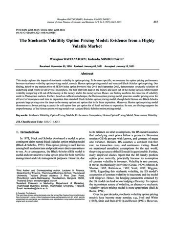
than 14 days to expiration increased from 66,925 (45,177) to 273,746 (86,622) contracts. Thecombined open interest (daily volume) for all options on that futures contract increased from92,083 (16,427) to 376,694 (32,820) contracts.We make two observations regarding liquidity. First, open interest for futures contractstends to peak when expiration is a couple of weeks away, after which open interest declinessharply. Second, among futures and options with more than a couple of weeks to expiration, thefirst six monthly contracts tend to be very liquid. Beyond approximately six months, liquidityis concentrated in the contracts expiring in March, June, September and December. Beyondapproximately one year, liquidity is concentrated in the contracts expiring in December. Due tothese liquidity patterns, we screen the available futures and options according to the followingprocedure: we discard all futures contracts with 14 or less days to expiration. Among theremaining, we retain the first six monthly contracts. Beyond these, we choose the first twocontracts with expiration in either March, June, September or December. Beyond these, wechoose the next four contracts with expiration in December. This procedure leaves us withtwelve generic futures contracts which we label M1, M2, M3, M4, M5, M6, Q1, Q2, Y1, Y2,Y3 and Y4.Figure 1 displays the futures data. The run-up in crude oil prices since 2002 is striking. Using the M1 futures contract as a proxy for the spot price, the Q2 futures contract isbackwardated 82.6 percent of the time and strongly backwardated 66.3 percent of the time.10Figure 2 displays the implied ATM log-normal volatilities for options on the first eight ofthe futures contracts.11 Volatility is evidently stochastic. The question is the extent to whichvolatility is unspanned.3Evidence of unspanned stochastic volatilityAs mentioned in the introduction, equilibrium and reduced-form models that derive futuresprices endogenously typically imply that volatility is spanned by the futures contracts. Thatis, changes in volatility can be hedged with a portfolio of futures contracts. In this section, we10Let S(t) denote the time-t spot price and F (t, T ) [P (t, T )] the time-t price of a futures contract [zero-couponbond] with maturity T t. The futures contract is backwardated if S(t) P (t, T )F (t, T ) 0 and stronglybackwardated if S(t) F (t, T ) 0. The numbers reported here are slightly lower than those reported inLitzenberger and Rabinowitz (1995) for an earlier sample.11At each date we choose the options that are closest to ATM. The options are American and we invert theirprices using the Barone-Adesi and Whaley (1987) formula. More details are given in Appendix B.6

investigate if that is indeed the case. Suppose we regress changes in volatility on the returns offutures contracts, the R2 s will indicate the extent to which volatility is spanned. However, thisapproach is not feasible since volatility is not directly observable. One alternative is to investigate how much of the variation in the prices of certain derivatives portfolios highly exposedto volatility (so-called “straddles”) can be explained by variation in the underlying futuresprices. Another alternative is to investigate how much of the variation in log-normal impliedvolatilities (which is related to expectations, under the risk-neutral measure, of future volatility) can be explained by variation in the underlying futures prices. We use both approachesto investigate the extent to which volatility is spanned. Although they are related, they dohave their relative strengths and weaknesses that we discuss below. Both approaches havepreviously been used by Collin-Dufresne and Goldstein (2002) and Heidari and Wu (2003) toinvestigate unspanned stochastic volatility in the fixed income market.12More specifically, we proceed in three steps. Suppose we have a set of contracts (futuresand their associated options), i 1, ., n. First, we factor analyze the covariance matrix ofthe daily futures returns and retain the first three principal components, P C f ut,1 , P C f ut,2 andP C f ut,3 . These summarize virtually all of the information in the futures returns.Second, for each futures contract i, we regress the daily return on the straddle that isclosest to ATM13 on the first three principal components of the futures returns as well as thesquared principal components and the cross-products between the principal components,14rtstraddle,i β0i β1i P Ctf ut,1 β2i P Ctf ut,2 β3i P Ctf ut,3 2 2 2β4i P Ctf ut,1 β5i P Ctf ut,2 β6i P Ctf ut,3 β7i P Ctf ut,1 P Ctf ut,2 β8i P Ctf ut,1 P Ctf ut,3 β9i P Ctf ut,2 P Ctf ut,3 ǫit .12(1)A third alternative is to investigate how much of the variation in realized volatility, estimated from high-frequency data, can be explained by variation in the underlying futures prices. Andersen and Benzoni (2005)use this approach to investigate unspanned stochastic volatility in the fixed income market. However, our dataset does not include high-frequency data for futures prices. A fourth alternative might be to use informationfrom variance swaps. However, these contracts are quite illiquid in the crude oil market.13We only search among straddles with moneyness (strike divided by the price of the underlying futurescontract) in the interval 0.95–1.05. Furthermore, we only consider options that have open interest in excess of100 contracts.14We add the squared principal components and the cross-products between the principal components tothe set of independent variables in the regressions in an attempt to take into account non-linearities in therelationship between straddle returns and futures returns.7

A straddle consists of a put option and a call option with the same strike. The price of anear-ATM straddle has low sensitivity to (small) variations in the price of the underlyingfutures contract (since “deltas” are close to zero for ATM straddles) but high sensitivity tovariations in volatility (since “vegas” peak for ATM straddles). Consequently, the extent towhich straddle returns can be explained by the principal components of the futures returnswill indicate the extent to which volatility is spanned by the futures contracts.For each futures contract i we also run regression (1) with the straddle return substitutedby the daily change in implied log-normal volatility.15 The implied log-normal volatility isrelated to the average expected (under the risk-neutral measure) log-normal volatility of theunderlying futures contract over the life of the option. Hence, these regressions also indicatethe extent to which volatility is spanned by the futures contracts.Third, we factor analyze the covariance matrix of the n time series of residuals from thestraddle return regressions and the implied volatility regressions. The principal componentsof the residuals are, by construction, independent of those of the futures returns. If thereis unspanned stochastic volatility in the data, we should see large common variation in theresiduals across option maturities. If the residuals are simply due to noisy data, we should notfind much common variation in the residuals.The advantage of running the regressions with straddle returns is that the results arenot conditional on a particular pricing model. The disadvantage is that even if volatility iscompletely unspanned by the futures contracts, the R2 s from the regressions will not necessarilybe close to zero. The reason is that straddle returns are highly convex in the futures returns(near-ATM straddles have high “gammas”), and we include the squared principal componentsof the futures returns in the regressions. Hence, some of the variation in straddle returns willbe explained by futures returns even if none of the variation in volatility can be explainedby the futures returns. In contrast, running the regressions with implied volatility shouldproduce R2 s close to zero if volatility is completely unspanned. However, in this case theresults will, to some extent, be conditional on the particular pricing model used for invertingimplied volatilities from option prices.An important issue is that our approach requires a full set of futures and straddle returns.The fact that the maturity range of futures and options has increased over the sample generates15The implied log-normal volatilities are computed as the averages of the implied log-normal volatilities ofthe puts and calls that constitutes the straddles. The options are American and we invert their prices usingthe Barone-Adesi and Whaley (1987) formula. More details are given in Appendix B.8

a tradeoff: as we include longer-term contracts in the analysis, we have fewer dates with a fullset of futures and straddle returns but obtain more information about common variation inresiduals across different option maturities. For this reason we perform the analysis with thefollowing five different sets of contracts: M1–M4, M1–M6, M1–Q2, M1–Y2 and M1–Y4.Table 1, Panel A, shows the adjusted R2 s from regressing straddle returns on the principalcomponents of the futures returns. The R2 s lie between 7.9 percent and 67.3 percent, indicatingthat it is very difficult to hedge volatility risk using futures contracts.16 Table 1, Panel B,shows the adjusted R2 s when replacing straddle returns with implied volatility changes in theregressions. In this case, the R2 s vary between 0.2 percent and 24.7 percent. This provideseven stronger evidence of the inability of futures contracts to hedge volatility risk.Table 2 displays the explanatory power of the first three principal components of theregression residuals. For the straddle return regressions, the first (second) principal componentexplains between 48.1 (12.3) percent and 79.5 (17.9) percent of the variation in the residualsacross maturities, while for the implied volatility regressions, it explains between 51.8 (12.7)percent and 79.4 (15.9) percent. The explanatory power of the third principal component ismostly in the single digits. Hence, there is large common variation in the residuals acrossoption maturities, which strongly indicates that the low R2 s from the regressions are mainlydue to a few unspanned volatility factors rather than noisy data.17,1816As discussed above, in these regressions the R2 s will not necessarily be close to zero even if volatility iscompletely unspanned. That the R2 s tend to decrease with straddle maturity is consistent with the fact that“gammas” of ATM straddles also decrease with maturity.17The correlation between the first principal component of the residuals from the straddle return regressionsand the first principal component of the residuals from the implied volatility regressions is consistently above0.95. Likewise for the second principal component.18A potential weakness of the procedure, as implemented here, is that the parameters in the regressionsare assumed constant over the entire sample. In reality we would expect the parameters to be time-varying.To take into account such time-variation, we have also performed the analysis using a rolling window of 100observations. The results are very similar to those reported here and therefore not included. However, they canbe found in the NBER working paper version of the article.9

4A model for commodity derivatives featuring unspanned stochastic volatilityBased on the evidence presented above, we now develop a tractable framework for pricingcommodity derivatives in the presence of unspanned stochastic volatility. In Sections 4.1 – 4.4,we present a general model, which nests some interesting, more parsimonious specificationsthat are described in Section 4.5.4.1The model under the risk-neutral measureLet S(t) denote the time-t spot price of the commodity with an instantaneous spot cost ofcarry given by δ(t). Furthermore, let y(t, T ) denote the time-t instantaneous forward costof carry at time T , with y(t, t) δ(t). Standard models of commodity derivatives, suchas Gibson and Schwartz (1990), Schwartz (1997), and Casassus and Collin-Dufresne (2005),among others, typically specify a process for S(t) and δ(t). Here instead, we follow Cortazarand Schwartz (1994) and Miltersen and Schwartz (1998), among others, and specify a processfor S(t) and y(t, T ); that is, we model the evolution of the entire forward cost of carry curve.The main theoretical contribution of this paper is to extend the framework to accommodateunspanned stochastic volatility. Specifically, we assume that the volatility of both S(t) andy(t, T ) may depend on two volatility factors, v1 (t) and v2 (t), and postulate the following verygeneral process for S(t), y(t, T ), v1 (t), and v2 (t) under the risk-neutral measure:dS(t)S(t)pv1 (t)dW1Q (t) σS2 v2 (t)dW2Q (t)ppdy(t, T ) µy (t, T )dt σy1 (t, T ) v1 (t)dW3Q (t) σy2 (t, T ) v2 (t)dW4Q (t)pdv1 (t) (η1 κ1 v1 (t) κ12 v2 (t))dt σv1 v1 (t)dW5Q (t)pdv2 (t) (η2 κ21 v1 (t) κ2 v2 (t))dt σv2 v2 (t)dW6Q (t), δ(t)dt σS1p(2)(3)(4)(5)where WiQ (t), i 1, ., 6, denote Wiener processes under the risk-neutral measure.19 Weallow W1Q (t), W3Q (t), and W5Q (t) to be correlated, with ρ13 , ρ15 , and ρ35 denoting pairwisecorrelations, and we also allow W2Q (t), W4Q (t), and W6Q (t) to be correlated, with ρ24 , ρ26 ,and ρ46 denoting pairwise correlations. This is the most general correlation structure thatpreserves the tractability of the model.19Existence of this process requires η1 0, η2 0, κ12 0, and κ21 0; see, e.g., the discussion of affineprocesses in Dai and Singleton (2000).10

The forward cost of carry is given by the forward interest rate minus the forward convenience yield, and the model could be extended with separate processes for the forward interestrate and the forward convenience yield.20 However, for pricing most commodity futures, thisextension is of minor importance; see, e.g., the discussion in Schwartz (1997). Furthermore, forpricing short-term or medium-term options on most commodity futures, the pricing error thatarises from not explicitly modelling stochastic

We also assess the importance of unspanned stochastic volatility when hedging an option portfolio. Hedging the option portfolio solely with futures contracts causes only a small re- . 5Eydeland and Geman (1998) propose a stochastic volatility Heston (1993) model for pricing energy deriva-tives. However, they only model the evolution of the .