Transcription
Stochastic modeling and optimization methods in InvestmentsICESAustin, September 2014Thaleia ZariphopoulouMathematics and IROMThe University of Texas at Austin
Financial MathematicsAn interdisciplinary field on the crossroads of stochastic processes,stochastic analysis, optimization, partial differential equations, finance,financial economics, decision analysis, statistics and econometricsIt studies derivative securities and investments,and the management of financial risksStarted in the 1970s with the pricing of derivative securities
Derivative securitiesDerivatives are financial contracts offering payoffs writtenon underlying (primary) assetsTheir role is to eliminate, reduce or mitigate risk
Major breakthroughBlack-Scholes-Merton 1973 The price of a derivative is the value of a portfolio that reproducesthe derivative’s payoff The components of this replicating portfolio yield the hedgingstrategiesThis idea together with Itô’s stochastic calculus started the field ofFinancial Mathematics Black, F. and M. Scholes (1973): The pricing of options andcorporate liabilities, JPE Itô, K. (1944): Stochastic integral, Proc. Imp. Acad. TokyoDöblin, W. (1940; 2000): Sur l’équation de Kolmogoroff, CRAS,Paris, 331
Louis Bachelier (1870-1946)Father of Financial MathematicsThesis: Théorie de la SpéculationAdvisor: Henri Poincaré
Louis Bachelier (1870-1946)Father of Financial MathematicsThesis: Théorie de la SpéculationAdvisor: Henri PoincaréBachelier model (1900)Wt a standard Brownian motion and µ, σ constantsincrement evolves asSt δ St µδ σ (Wt δ Wt )Bachelier’s work was neglected for decadesIt was not recognized until Paul Samuelson introduced it to Economics
Samuelson model (1965)log-normal stock pricesdSs µSs ds σSs dWswidely used in finance practiceEuropean callCt0tinitiation(ST K ) Texercise
Replication (Black-Scholes-Merton) Market: stock S and a bond B (dBs rBs ds) Find a pair of stochastic processes (αs , βs ) , t s T , such that a.s.at T ,αT ST βT BT (ST K ) The derivative price process Cs , t s T , is then given byCs αs Ss βs Bs Price at initiation: Ct αt St βt Bt Hedging strategies: (αs , βs ) , t s T
Replication using self-financing strategiesCs Ct Z stαu dSu Z stβu dBu Postulate a price representation Cs h (Ss , s) for a smooth function h(x, t) Itô’s calculus Z s tCs h (St , t)1ht (Su , u) µSu hx (Su , u) σ 2 Su2 hxx (Su , u) du2 Z stσSu hx (Su , u) dWuP
Black and Scholes pdeThe function h (x, t) solves1rh ht σ 2 x 2 hxx rxhx2with h (0, t) 0 and h (x, T ) (x K ) European call price processCs h (Ss , s)Hedging strategiesh (Ss , s) hx (Ss , s) Ss(αs , βs ) hx (Ss , s) ,Bs
A universal pricing theoryfor general price processes (semimartingales)
Arbitrage-free pricing of derivative securitiesHarrison, Kreps, Pliska (1979,1981)ArbitrageA market admits arbitrage in [t, T ] if the outcome XT of self-financingstrategies satisfies Xt 0, andP (XT 0) 1 and P (XT 0) 0In arbitrage-free markets, derivative prices are given byC t EQ BτCτ FtBt Q P under which (discounted) assets are martingalesModel-independent pricing theoryP Q EQ ( · Ft )Linear pricing rule and change of measure
Mathematics and derivative securities Martingale theory and stochastic integrationDerivative prices are martingales under QHedging strategies are the integrands (martingale representation) Malliavin calculus for sensitivities (”greeks”) Markovian models - (multi-dim) linear partial differential equationsEarly exercise claims - optimal stopping, free-boundary problemsExotics - linear pde with singular boundary conditions Credit derivatives - copulas, jump processes Bond pricing, interest rate derivatives, yield curve: linear stochasticPDE
Some problems of current interest Stochastic volatility Correlation, causality Systemic risk Counterparty risk Liquidity risk, funding risk Commodities and Energy Calibration Market data analysis.
The other side of Finance: Investments
Derivative securities and investmentsWhile in derivatives the aim is to eliminate the risk, the goal ininvestments is to profit from it Derivatives industry uses highly quantitative methods Academic research and finance practice have been working together,especially in the 80s and 90s Traditional investment industry is not yet very quantitative A unified ”optimal investment” theory does not exist to date Ad hoc methods are predominantly usedDisconnection between academic research and investment practice
CriterionMarket opportunitiesutilityrisk measuresrisk premiaP, ambiguity re g timesmarket signalsshortsellingdrawdown, leverage
Academic research in investments
Modeling investor’s behaviorUtility theory Created by Daniel Bernoulli (1738) responding to his cousin,Nicholas Bernoulli (1713) who proposed the famous St. Petersburgparadox, a game of ”unreasonable” infinite value based on expectedreturns of outcomes D. Bernoulli suggested that utility or satisfaction has diminishingmarginal returns, alluding to the utility being concave (see, also,Gabriel Cramer (1728)) Oskar Morgenstern and John von Neumann (1944) published thehighly influential work “Theory of games and economic behavior”.The major conceptual result is that the behavior of a rational agentcoincides with the behavior of an agent who values uncertain payoffsusing expected utility
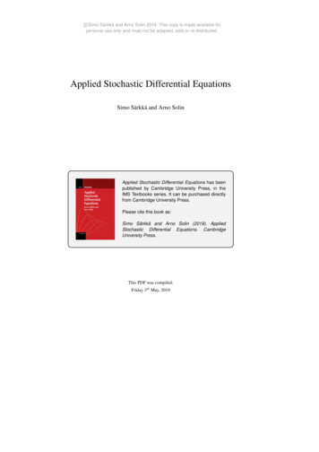
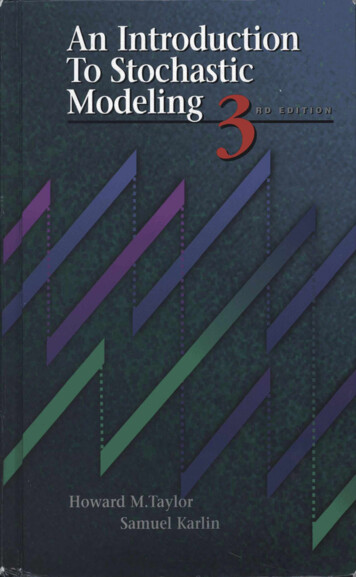
Utility function and its marginalU 0(x)U (x)0x0xInada conditions: lim U 0(x) and lim U 0(x) 0x x 0xU 0 (x) 1x U (x)Asymptotic elasticity: lim
Stochastic optimizationand optimal portfolio construction
Merton’s portfolio selection continuous-time model start at t 0 with endowment x,market (Ω, F, (Ft ) , P) , price processes follow investment strategies, πs Fs , t s T map their outcome XTπ EP ( U (XTπ ) Ft , Xtπ x) maximize terminal expected utility (value function)V (x, t) sup EP ( U (XTπ ) Ft , Xtπ x)πR. Merton (1969): Lifetime portfolio selection under uncertainty: thecontinuous-time case, RES
Stochastic optimization approachesMarkovian modelsNon-Markovian modelsDynamic Programming PrincipleBellman (1950)Duality approachBismut (1973)
Markovian modelsStock price: dSt St µ (Yt , t) dt St σ (Yt , t) dWtStochastic factors: dYt b (Yt , t) dt a (Yt , t) d W̃t ; correlation ρControlled diffusion (wealth): dXsπ πs µ (Yt , t) dt πs σ (Ys , s) dWs , Xt xDynamic Programming Principle (DPP)V (Xsπ , Ys , s) sup EP V Xsπ0 , Ys0 , s 0 Fs πHamilton-Jacobi-Bellman equation1 2 2Vt maxπ σ (y, t) Vxx π (µ (y, t) Vx σ (y, t) a (y, t) Vxy )π R21 a 2 (y, t) Vyy b (y, t) Vy 0,2with V (x, y, T ) U (x)
Optimal portfolios (feedback controls)π (x, y, t) a (y, t) Vxyµ (y, t) Vx ρσ 2 (y, t) Vxxσ (y, t) Vyyπs π (Xs , Ys , s) and dXs πs µ (Yt , t) dt πs σ (Ys , s) dWsDifficulties set of controls non-compact, state-constraints degeneracies, lack of smoothness, validity of verification theorem value function as viscosity solution of HJB, smooth cases for specialexamples existence, smoothness and monotonicity properties of π (x, y, t) probabilistic properties of optimal processes πs , Xs and their ratioKaratzas, Shreve, Touzi, Bouchard, Pham, Z.,.
Duality approachin optimal portfolio construction
Dual optimization problem - utility convex conjugateŨ (y) max (U (x) xy)x 0 Introduced in stochastic optimization by Bismut (1973) Introduced in optimal portfolio construction by Bismut (1975) andFoldes (1978) Further results by Karatzas et al (1987) and Cox and Huang (1989) Xu (1990) shows that the HJB linearizes for complete markets Kramkov and Schachermayer (1999) establish general results forsemimartingale models
Semimartingale stock price modelsH : predictable processes integrable wrt the semimartingale SX (x) X : Xt x nRt0Hs · dSs , t [0, T ] , H HoY {Y 0, Y0 1, XY semimartingale for all X X }Y (y) yY, y 0Asymptotic elasticity condition: lim supx Primal problemu (x) sup EP (U (XT ))X X (x) xU 0 (x)U (x) 1Dual problemũ (y) infY Y(y)EP Ũ (YT )
Duality results for semimartingale stock price modelsIf u (x) , for some x, and ũ (y) for all y 0, then: ũ (y) sup (u (x) xy)x 0dQdPQ M (S)martingale measures Q P ũ (y) infe EP Ũ y , y 0, with Me (S) the set of if Q optimal, the terminal optimal wealth (primal problem) XTx, is given by dQ U 0 XTx, u 0 (x)dPKramkov and Schachermayer, Karatzas, Cvitanic, Zitkovic, Sirbu, .
Some extensions
Coupled stochastic optimization problemsSystems of HJB equationsDelegated portfolio managementfees, capitalinvestor manager investorrisk, returnmanagermV i (x, t) sup EP U i XT , It s T AiiV m (y, t) sup EP U m YT , It s T Am Ft , X t x Gt , Yt y I m and I i : inputs from the manager (performance, risk taken)and the investor (investment targets)Benchmarking and asset specialization among competing fund managersV 1 (x, t) sup EP1 ( U1 (XT , YT ) Ft , Xt x)A1V 2 (y, t) sup EP2 ( U2 (YT , XT ) Gt , Yt y)A2
Proportional transaction costs N stocks, one riskless bond Pay proportionally αi for sellingand β i for buying the i th stock Xs : bond holding, Ys Ys1 , ., YsN : stock holdings, t s T ,iiNiidXs rXs ds ΣNi 1 α dMs Σi 1 β dLsdYsi µi Ysi ds σ i Ysi dWsi dLsi dMsiVariational inequalities with gradient constraintsmin Vt L(y1 ,.yN ) V rxVx , a 1 Vx Vy1 , β 1 Vx Vy1 ,. a N Vx VyN , β N Vx VyN 0,iNiwith V (x, y1 , .yN , T ) U x ΣNi 1 α yi 1{yi 0} Σi 1 β yi 1{yi 0}
Liquidation of financial positions and price impactbig investor : delegates liquidation to ”major agent”major agent : liquidates in the presence of many small agentssmall agents: noise traders and high-frequency tradersOptimal liquidation is an interplay between speed and volumeToo fastToo slow price impactunfavorable price fluctuationsMean-field games Aggregate impact from noise traders Aggregate impact from high-frequency traders
Model uncertaintyand optimal portfolio construction
Knightian uncertainty (model ambiguity)Frank Knight (1921)The historical measure P might not be a priori known Gilboa and Schmeidler (1989) built an axiomatic approach forpreferences towards both risk and model ambiguity. They proposedthe robust utility formXTπ inf EQ (U (XTπ )) ,Q Qwhere U is a classical utility function and Q a family of subjectiveprobability measuresStandard criticism: the above criterion allows for very limited , if at all,differentiation of models with respect to their plausibility
Knightian uncertainty Maccheroni, Marinacci and Rustichini (2006) extended the aboveapproach toXTπ inf (EQ (U (XTπ )) γ (Q))Q Qwhere the functional γ (Q) serves as a penalization weight to eachQ-market modelEntropic penalty and entropic robust utilityγ (Q) H ( Q P)with H ( Q P) ZdQdQlndPdPdP inf (EQ (U (XTπ )) γ (Q)) ln EP e U (XT ) Q QHansen, Talay, Schied, Föllmer, Frittelli, Weber .
Maxmin stochastic optimization problemStock dynamics: St St1 , ., Std , t [0, T ] , semimartingales Wealth dynamics: Xtα x Objective:v (x) supRt0αs · dSs , Xtα 0, t 0inf (EQ (U (XT )) γ (Q)) ,X X (x) Q Qwhere Q { Q P γ (Q) }Duality approachu (y) infinfY YQ (y) Q Qwhere Ũ (y) sup (U (x) xy)x 0 EQ Ũ (YT ) γ (Q)
Investment practice
Portfolio selection criteriaSingle-period criteria Mean-variance maximize the mean return for fixed variance Black-Litterman allows for subjective views of the investorLong-term criterion Kelly criterion maximize the long-term growthWhile using these criteria allows for tractable solutions, they havemajor deficiencies and limitations which do not capture importantfeatures like the evolution of both the market and the investor’stargets
Mean–variance optimization
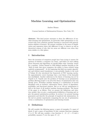
Harry Markowitz (1952)Performance of portfolio returns mean, variance Single period: 0, T Allocation weights at t 0: a (a 1 , · · · , a n );Pni 1 ai 1 n1 ,··· ,R Asset returns: RT RTTa Return on allocation: RTPni 1 ai RiTMean–variance optimizationFor a fixed acceptable variancev maximize the mean,a:maxPiai 1a vVar(RT)aEP (RT)For a fixed desired mean mminimize the variance,ora:minPiai 1a mEP (RT)aVar (RT)
Efficient frontier0.120.100.08µa 0.060.040.020.000.050.100.15σa0.200.25
Despite its popularity and wide use,MV has major deficiencies ! Model error and unstable solutions Time–inconsistency of optimal portfolios Dynamic extensions not available to date
Model error and unstable solutions Quality and availability of market data not always good Estimation error very high Optimal allocation highly sensitive to this error Historical returns frequently used, not “forward–looking” Optimal portfolios are frequently “extreme”, unnatural, highshort–selling Asset managers are familiar with only certain asset classes and sectors(“familiarity versus diversification” issue)Some of these issues can be partially addressed by theBlack–Litterman criterion which adjusts the equilibrium assetreturns by the manager’s individual views on “familiar” assets(classes or sectors)
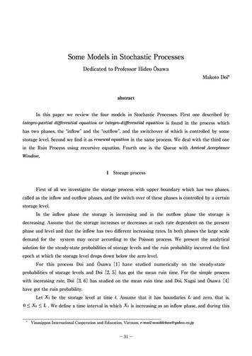
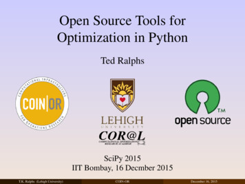
Time–inconsistency of MV problemAt time t 0v0 2Ta0*,0aT*,00T2TAt time t TvT 2T v0 2T0aT*,T6 aT*,0TGame theoretic approach (Björk et al. (2014))2T
Dynamic (rolling investment times) MV optimizationv0 T0vT 2TTv2T 3T2T3T This problem is not the same as setting, at t 0, the “three–period”variance target v0 3T Is there a discrete process v0 2T , vT 2T , · · · , vnT (n 1)T , · · ·modelling the targeted conditional variance (from one period to thenext) that will generate time–consistent portfolios? What is the continuous–time limit of this construction? Can it be addressed by mapping the MV problem to thetime–consistent expected utility problem? No! because the expectedutility approach produces a solution “backwards in time”!
Can the theoretically foundational approach ofexpected utility meet the investment practice?
MV and expected utilityTheoryPracticeCriteriaRisk–return tradeoff practical but stilldoes not capture muchUtility is an elusive conceptDifficult to quantify, especially forlonger horizonsEvolutiontime–inconsistenttime consistent (semigroup property)sequential ad hoc implementationbackward construction (DPP)captures info up to now, limited andad hocrequires forecasting of asset returns,major difficultiessingle–periodinflexible investment horizonSimilar limitations and discrepancies arise between expected utility, and theBlack-Litterman and Kelly criteria. Practical features of these industry criteria donot fit in the expected utility framework, which however has major deficiencies
Such issues and considerations prompted the development of theforward investment performance approach (Musiela and Z., 2002- )
Market environment (Ω, F, (Ft ), P) ;W (W 1 , . . . , W d ) Traded securities(dSti Sti µit dt σti · dWt , dBt rt Bt dt ,S0i 0,B0 11 i kµt , rt R, σti Rd bounded and Ft -measurable stochastic processes Wealth process dXtπ σt πt · (λt dt dWt ) Postulate existence of an Ft -measurable stochastic process λt Rdsatisfyingµt rt 11 σtT λt No assumptions on market completeness
Forward investment performance processOptimality across timesoptimality across trading timesU (x, t) Ft 0 U (x, s) Fs 0U (x, t) Ft π π , t) Fπ x)U (x,s) s) supEP (U, sX U (x,sup(X(Xs, sXA E(Us x)t ,tt) FAWhatsuchis thea meaningthis process? Doesprocess ofawaysexist? IsDoesit unique?such a process aways exist? Axiomatic construction?Is it doesunique? Howit relate to criteria in investment practice? Axiomatic construction?8
Forward investment performance processU (x, t) is an Ft -adapted process, t 0 The mapping x U (x, t) is strictly increasing and strictly concave For each self-financing strategy π and the associated (discounted)wealth XtπEP (U (Xtπ , t) Fs ) U (Xsπ , s),0 s t There exists a self-financing strategy π and associated (discounted) wealth Xtπ such thatEP (U (Xtπ , t) Fs ) U (Xsπ , s), 0 s t
The forward performance SPDE
The forward performance SPDE (MZ 2007)Let U (x, t) be an Ft measurable process such that the mappingx U (x, t) is strictly increasing and concave. Let also U (x, t) be thesolution of the stochastic partial differential equationdU (x, t) 1 σσ A (U (x, t)λ a)2A2 U (x, t)2dt a(x, t) · dWt where a a (x, t) is an Ft adapted process, and A x. Then U (x, t)is a forward performance process.Once the volatility is chosen the drift is fully specified if we know (σ, λ)
The volatility of the investment performance processThis is the novel element in the new approach The volatility models how the current shape of the performanceprocess is going to diffuse in the next trading period The volatility is up to the investor to choose, in contrast to theclassical approach in which it is uniquely determined via the backwardconstruction of the value function process In general, a(x, t) F (x, t, U , Ux , Uxx ) may depend on t, x, U , itsspatial derivatives etc. When the volatility is not state-dependent, we are in the zerovolatility caseSpecifying the appropriate class of volatility processes is a centralproblem in the forward performance approachMusiela and Z., Nadtochiy and Z., Nadtochyi and Tehranchi, Berrier etal., El Karoui and M’rad
The zero volatility case: a(x, t) 0
Time-monotone performance processThe forward performance SPDE simplifies todU (x, t) The process1 σσ A (U (x, t)λ)dt2A2 U (x, t)2U (x, t) u (x, At )with At Z t0 λs 2 dsand u(x, t) a strictly increasing and concave w.r.t. x function solvingut is a solutionMZ (2006, 2009)Berrier, Rogers and Tehranchi (2009)1 ux22 uxx
Optimal wealth and portfolio processesand a fast diffusion equation
Local risk tolerance function and a fast diffusion equation1rt r 2 rxx 02ux (x, t)r(x, t) uxx (x, t)System of SDEs at the optimumRt , r(Xt , At ) andThen(At Z t0 λs 2 dsdXt Rt λt · (λt dt dWt )dRt rx (Xt , At )dXt and the optimal portfolio isπt Rt σt λt
Complete constructionutility inputs, heat eqn and fast diffusion eqnut 1 ux22 uxx 1ht hxx 021rt r 2 rxx 02 positive solutions to heat eqn and Widder’s thmhx (x, t) Z1 2e xy 2 y t ν (dy)Roptimal wealth processXt ,x h h ( 1)(x, 0) At Mt , At M Z t0λs ·dWs ,hM it Atoptimal portfolio processπt ,x r(Xt , At )σt λt hx h ( 1) Xt ,x , At , At σt λt
Forward performance approach underKnightian uncertainty
Forward robust portfolio criterion(Kallbald, Oblój, Z.) allow flexibility with respect to the investment horizon incorporate ”learning” produce optimal investment strategies closer to the ones used inpracticeForward robust criterionA pair (U (x, t) , γt,T (Q)) of a utility process and a penalty criterionwhich satisfies, for all 0 t T ,U (x, t) ess sup ess infαQ Qt,TEQU (x Z Ttαs · dSs , T ) Ft!! γt,T (Q)with QT {Q Q : Q FT P FT }This criterion gives rise to an ill-posed SPDE corresponding to azero-sum stochastic differential game
Connection with the Kelly criterion
Is there a pair (U (x, t) , γt,T ) that yields the Kelly optimal-growthportfolio?“True” model dSt St λ t dt σt dWt1 , (W 1 , W 2 ) under P“Proxy” model: dSt St λ̂t dt σt d Ŵt1 , (W 1 , W 2 ) under P̂ For each Q P̂ and each T 0, let ηt (ηt1 , ηt2 ), 0 t T ,dQ Z ·Z ·ηs2 d Ŵs2 Doléans-Dade exponential: E (Y )t exp Yt 12 hY it d P̂FT E0ηs1 d Ŵs1 0 TCandidate penalty functionalsγt,T (Q) EQZ Ttg(ηs , s)ds Ft!
Logarithmic risk preferencesand quadratic penalty1U (x, t) ln x 2Z t0γt,T (Q ) EQ ηηδsλ̂2 ds,1 δs sZ Tδst2t 0, x 0 ηs ds Ft!2 The process δt is adapted, non–negative and controls the strengthof the penalization It models the confidence of the investor re the ”true” model
(Fractional) Kelly strategies and forward optimal controlsInvestor chooses proxy model (λ̂t ) and confidence level (δt )Optimal measure Q ηηt !λ̂t ,0(1 δt )anddQ ηd P̂ E Z ·0λ̂td Ŵt11 δt!TOptimal forward Kelly portfolioπ̄t δt λ̂t1 δt σt If δt (infinite trust in the estimation), then π̄t λ̂σtt , which is theKelly strategy associated with the most likely model P̂ If δt 0 (no trust in the estimation), then π̄t 0 and the optimalbehavior is to invest nothing in the stock
Open problemsAcademic researchInvestment practicestudy of forward SPDEreconcile with MVforward, dynamic constructionexistence and uniquenessfor concave, increasing slnscharacterize admissiblevolatility processesForward performanceapproachreconcile with Black-Littermaninject manager’s views inthe forward volatility and driftapprox. of slns via finite-dimMarkovian multi-factor processesreconcile with Kelly criterionmodel ambiguity andand fractional Kellyergodic properties ofportfolios and wealth processesprovide a normative platform toconnect these three criteria
Financial Mathematics An interdisciplinary field on the crossroads of stochastic processes, stochastic analysis, optimization, partial differential equations, finance, financial economics, decision analysis, statistics and econometrics It studies derivative securities and investments, and the management of financial risks