Transcription
Distributed Deep Q-LearningKevin Chavez1 , Hao Yi Ong1 , and Augustus Hong1Abstract— We propose a distributed deep learning modelto successfully learn control policies directly from highdimensional sensory input using reinforcement learning. Themodel is based on the deep Q-network, a convolutional neuralnetwork trained with a variant of Q-learning. Its input israw pixels and its output is a value function estimatingfuture rewards from taking an action given a system state.To distribute the deep Q-network training, we adapt theDistBelief software framework to the context of efficientlytraining reinforcement learning agents. As a result, the methodis completely asynchronous and scales well with the numberof machines. We demonstrate that the deep Q-network agent,receiving only the pixels and the game score as inputs, was ableto achieve reasonable success on a simple game with minimalparameter tuning.I. I NTRODUCTIONReinforcement learning (RL) agents face a tremendouschallenge in optimizing their control of a system approachingreal-world complexity: they must derive efficient representations of the environment from high-dimensional sensoryinputs and use these to generalize past experience to newsituations. While past work in RL has shown that with goodhand-crafted features agents are able to learn good controlpolicies, their applicability has been limited to domainswhere such features have been discovered, or to domainswith fully observed, low-dimensional state spaces [1]–[3].We consider the problem of efficiently scaling a deeplearning algorithm to control a complicated system withhigh-dimensional sensory inputs. The basis of our algorithmis a RL agent called a deep Q-network (DQN) [4], [5] thatcombines RL with a class of artificial neural networks knownas deep neural networks [6]. DQN uses an architecture calledthe deep convolutional network, which utilizes hierarchicallayers of tiled convolutional filters to exploit the local spatialcorrelations present in images. As a result, this architectureis robust to natural transformations such as changes ofviewpoint and scale [7].In practice, increasing the scale of deep learning withrespect to the number of training examples or the number ofmodel parameters can drastically improve the performance ofdeep neural networks [8], [9]. To train a deep network withmany parameters on multiple machines efficiently, we adapta software framework called DistBelief to the context of thetraining of RL agents [10]. Our new framework supportsdata parallelism, thereby allowing us to potentially utilizecomputing clusters with thousands of machines for largescale distributed training, as shown in [10] in the context of1 K.Chavez, H. Y. Ong, and A. Hong are with the Departments of Electrical Engineering, Mechanical Engineering, and Computer Science, respectively, at Stanford University, Stanford, CA 94305, USA fkjchavez,haoyi, auhongg@stanford.eduunsupervised image classification. To achieve model parallelism, we use Caffe, a deep learning framework developedfor image recognition that distributes training across multipleprocessor cores [11].The contributions of this paper are twofold. First, wedevelop and implement a software framework adapted thatsupports model and data parallelism for DQN. Second, wedemonstrate and analyze the performance of our distributedRL agent. The rest of this paper is organized as follows.Section II introduces the background on the class of machinelearning problem our algorithm solves. This is followed bySection III and Section IV, which detail the serial DQNand our approach to distributing the training. Section Vdiscusses our experiments on a classic video game, and someconcluding remarks are drawn and future works mentionedin Section VI.II. BACKGROUNDWe begin with a brief review on MDPs and reinforcementlearning (RL).A. Markov decision processIn an MDP, an agent chooses action a t at time t afterobserving state s t . The agent then receives reward r t , andthe state evolves probabilistically based on the current stateaction pair. The explicit assumption that the next state onlydepends on the current state-action pair is referred to as theMarkov assumption. An MDP can be defined by the tuple.S; A; T; R/, where S and A are the sets of all possiblestates and actions, respectively, T is a probabilistic transitionfunction, and R is a reward function. T gives the probabilityof transitioning into state s 0 from taking action a at thecurrent state s, and is often denoted T .s; a; s 0 /. R gives ascalar value indicating the immediate reward received fortaking action a at the current state s and is denoted R .s; a/.To solve an MDP, we compute a policy ? that, iffollowed, maximizes the expected sum of immediate rewardsfrom any given state. The optimal policy is related to theoptimal state-action value function Q? .s; a/, which is theexpected value when starting in state s, taking action a,and then following actions dictated by ? . Mathematically,it obeys the Bellman recursionX Q? .s; a/ D R .s; a/ CT s; a; s 0 maxQ? s 0 ; a0 :0s 0 2Sa 2AThe state-action value function can be computed using adynamic programming algorithm called value iteration. To
obtain the optimal policy for state s, we computerectifier nonlinearity ? .s/ D argmax Q? .s; a/ :f .x/ D max .0; x/ ;a2Awhich was empirically observed to model real/integer valuedinputs well [12], [13], as is required in our case. Theremaining layers are fully-connected linear layers with asingle output for each valid action. The number of validactions varies with the game application. The neural networkis implemented on Caffe [11], which is a versatile deeplearning framework that allows us to define the networkarchitecture and training parameters freely. And becauseCaffe is designed to take advantage of all available computing resources on a machine, we can easily achieve modelparallelism using the software.B. Reinforcement learningThe problem reinforcement learning seeks to solve differsfrom the standard MDP in that the state space and transitionand reward functions are unknown to the agent. The goal ofthe agent is thus to both build an internal representation ofthe world and select actions that maximizes cumulative futurereward. To do this, the agent interacts with an environmentthrough a sequence of observations, actions, and rewards andlearns from past experience.In our algorithm, the deep Q-network builds its internalrepresentation of its environment by explicitly approximatingthe state-action value function Q? via a deep neural network.Here, the basic idea is to estimateB. Q-learningWe parameterize the approximate value functionQ .s; a j / using the deep convolutional network asdescribed above, in which are the parameters of theQ-network. These parameters are iteratively updated by theminimizers of the loss functionhi.yi Q .s; aI i //2 ;Li . i / D E(1)Q? .s; a/ D max E ŒR t j s t D s; a t D a; ; where maps states to actions (or distributions over actions),with the additional knowledge that the optimal value functionobeys Bellman equation ? 0 0Q .s; a/ D 0E r C maxQ s ; a j s; a ;0s Es;a . /awithiterationnumberi,targetyi DEs 0 E Œr C maxa0 Q .s 0 ; a0 I i 1 / j s; a ,and“behaviordistribution” (exploration policy .s; a/. The optimizers ofthe Q-network loss function can be computed by gradientdescentwhere E is the MDP environment.III. A PPROACHThis section presents the general approach adapted fromthe serial deep Q-learning in [4], [5] to our purpose. Inparticular, we discuss the neural network architecture, theiterative training algorithm, and a mechanism that improvestraining convergence stability.Q .s; aI / WD Q .s; aI / C r Q .s; aI / ;with learning rate .For computational expedience, the parameters are updatedafter every time step; i.e., with every new experience. Ouralgorithm also avoids computing full expectations, and wetrain on single samples from and E. This results in theQ-learning update 0 0.s;Q .s; a/ WD Q .s; a/ C r C maxQs;aQa/:0A. Preprocessing and network architectureWorking directly with raw video game frames can becomputationally demanding. Our algorithm applies a basicpreprocessing step aimed at reducing the input dimensionality. Here, the raw frames are gray-scaled from their RGBrepresentation and down-sampled to a fixed size for inputto the neural network. For this paper, the function appliesthis preprocessing to the last four frames of a sequence andstacks them to produce the input to the state-action valuefunction Q.We use an architecture in which there is a separate outputunit for each possible action, and only the state representationis an input to the neural network; i.e., the preprocessed fourframes sequence. The outputs correspond to the predictedQ-values of the individual action for the input size. Themain advantage of this type of architecture is the ability tocompute Q-values for all possible actions in a given statewith only a single forward pass through the network. Theexact architecture is presented in Appendix A, but a briefoutline is as follows. The neural network takes as input asequence of four frames preprocessed as described above.The first few layers are convolutional layers that applies aaThe procedure is an off-policy training method [14] thatlearns the policy a D argmaxa Q .s; aI / while using anexploration policy or behavior distribution selected by an -greedy strategy.The target network parameters used to compute y inEq. (1) are only updated with the Q-network parametersevery C steps and are held fixed between individual updates.These staggered updates stabilizes the learning process compared to the standard Q-learning process, where an updatethat increases Q .s t ; a t / often also increases Q .s tC1 ; a/for all a and hence also increases the target y. Theseimmediate updates could potentially lead to oscillations oreven divergence of the policy. Deliberately introducing adelay between the time an update to Q is made and the timethe update affects the targets makes divergence or oscillationsmore unlikely [4], [5].2
Algorithm 1 Worker k: ComputeGradientOstate: Replay dataset Dk , game state s t , target model ,target model generation C. Experience replayReinforcement learning can be unstable or even divergewhen a nonlinear function approximator such as a neuralnetwork is used to represent the value function [15]. Thisinstability has several causes. A source of instability is thecorrelations present in the sequence of observations. Additionally, the fact that small updates to Q may significantlychange the policy and therefore change the data distribution.Finally, the correlations between Q and its target valuescan cause the learning to diverge. [4], [5] address theseinstabilities uses a mechanism called experience replay thatrandomizes over the data, thereby removing correlations inthe observation sequence and smoothing over changes in thedata distribution.In experience replay, the agent’s experiences at each timestep is stored as a tuple e t D .s t ; a t ; r t ; s tC1 / in a datasetD t D .e1 ; : : : ; e t / pooled over many game instances (definedby the start and termination of a game) into a replay memory.During the inner loop of the algorithm, we apply Q-learningupdates, or minibatch updates, to samples of experiencedrawn at random from the replay dataset.This approach demonstrates several improvements overstandard Q-learning. First, each step of experience is potentially used in many weight updates, thus allowing for greaterdata efficiency. Second, learning directly from consecutivesamples is inefficient due to the strong correlations betweenthe samples. Randomizing the samples breaks these correlations and reduces the update variance. Last, when learningon-policy the current parameters determine the next datasample that the parameters are trained on. For instance, if themaximizing action is to move left then the training sampleswill be dominated by samples from the left-hand side; if themaximizing action then changes to the right then the trainingdistribution will also change. Unwanted feedback loops maytherefore arise and the method could get stuck in a poor localminimum or even diverge.With experience replay, the behavior distribution is averaged over many of its states, smoothing out learning andavoiding oscillations or divergence in the parameters. Notethat when learning by experience replay, it is necessary tolearn off-policy because our current parameters are differentto those used to generate the sample, which motivates thechoice of Q-learning. In practice, our algorithm only storesthe last N experience tuples in the replay memory. It thensamples uniformly at random from D when performingupdates. This approach is limited because the memory bufferdoes not differentiate important transitions and always overwrites with recent transitions owing to the finite memory sizeN . Similarly, the uniform sampling gives equal importanceto all transitions in the replay memory. A more sophisticatedsampling strategy might emphasize transitions from whichwe can learn the most, similar to prioritized sweeping [16].Fetch model and iteration number n from server.if n C then O bn C c C 1max f.Nmax n/ Nmax ; 0g.1 q/ mi n C q max maxa Q . .s t / ; aI / w.p. 1 Select action a t Drandom actionotherwiseExecute action a t and observe reward r t and frame x t C1Append s t C1 D .s t ; a t ; x tC1 / and preprocess tC1 D.s t C1 /Store experience . t ; a t ; r t ; t C1 / in DkUniformly sample minibatch of experiences X from Dk , where Xj D j ; aj ; rj ; j C1 rj if j C1 terminalSet yj D0OOrj C maxa0 Q j C1 ; a I otherwiseq b r f . I X/ D1Xr bi D1 1.Q. i ; ai I /2yi /2Send to parameter server.Algorithm 2 Distributed deep Q-learningfunction RMSP ROP U PDATE( )ri0:9ri C 0:1 . /2i for all iAcquire write-lockp i i . /i riRelease write-lockInitialize server i N .0; /, r0, n 0for all workers k doAsyncStartPopulate Dk by playing with random actionsrepeatC OMPUTE G RADIENTuntil server timeoutAsyncEndwhile n MaxIters doif latest model requested by worker k thenAcquire write-lockSend . ; n/ to worker kRelease write-lockif gradient received from worker k thenRMSP ROP U PDATE( )n nC1IV. D ISTRIBUTED DEEP Q- LEARNINGAlgorithm 1 and Algorithm 2 define the distributed deepQ-learning algorithm. In this section we discuss some important points about parallelism and performance.Shutdown server3
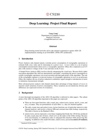
gradient computation on each of the worker machines. Caffeallows us to take advantage of fast BLAS implementations,using the worker’s CPU or GPU resources.In this sense, the work done by a single node is alsoparallelized—either across multiple CPU cores or many GPUcores. Pushing the computation down to the GPU yields asubstantial speed up, but it further constrains the size of themodel. The GPU memory must not only hold the modeland batch of data, but also all the intermediate outputs ofthe feedforward computation. This memory limit is oftenapproached in practice, especially for lower end GPUs. TheCPU’s memory is much more accommodating and should beable to hold any reasonably large model. In the case wherethe worker computation must be done on the CPU due tomemory constraints, the advantages of distributed deep Qare even more drastic.A. Data parallelismThe serial Deep Q-learning algorithm uses stochastic gradient descent to train the Q network. SGD is an inherentlysequential algorithm, but various attempts have been madeto parallelize it effectively. We implement Downpour SGD,as presented in [10]. A parameter server stores a global copyθ : θ αθΔθθC. Communication patternThe server must communicate with all workers since eachrequires the latest model at every iteration. Each worker, inturn, communicates with the server to send a gradient, butdoes not need to communicate with any other worker node.This is similar to a one-to-all and all-to-one communicationpattern, which could benefit from the allreduce primitive.However, all of the communication happens asynchronously,breaking the allreduce communication pattern. Further,to minimize the “staleness” of the model used by a worker forits gradient computation, it should fetch the latest version ofthe model directly from the server, not in bit-torrent fashionfrom its peers.Fig. 1: A graphic representation of Downpour SGD developed in [10].of the model. Each worker node is responsible for:1) Fetching the latest model, , from the server2) Generating new data for its local shard3) Computing a gradient using this model and mini-batchfrom its local replay memory dataset4) Sending the gradient back to the serverThese operations constitute a single worker iteration.All workers perform these iterations independently, asynchronously fetching from and pushing to the parameterserver. Upon receiving a gradient, the parameter serverimmediately applies an update to the global model. The onlysynchronization is a write-lock on the model as it is beingwritten to the network buffer.For typical sizes of Q-networks, it takes much longer tocompute a mini-batch gradient than it does to perform aparameter update. Therefore we can train on more data inthe same amount of time by simply adding worker nodes(eventually this breaks, as we discuss later). Since eachmini-batch is supposed to be drawn uniformly at randomfrom some history of experiences, we can keep completelyindependent histories on each of the worker nodes andsample only from the local dataset. This allows our algorithmto scale extremely well with the size of the training data.D. Scalability issuesAs we scale up the number of worker nodes, certainissues become increasingly important in thinking about theperformance of the distributed deep Q-learning algorithm.1) Server bottleneck: With few machines, the speed oftraining is bound by the gradient computation time. In thisregime, the frequency of parameter updates grows linearlywith the number of workers. However, the server takes somefinite amount of time, , to receive a gradient message andapply a parameter update. Thus, even with an infinite poolof workers, we cannot perform more than 1 updates persecond.This latency, , is generally small compared to the gradientcomputation time, but it becomes more significant as thenumber of workers increases. Suppose a mini-batch gradientcan be computed in time T . A pool of P workers will—on average—serve up a new gradient every T P . Thus,once we have P D T workers, we will no longer see anyimprovement by adding nodes.This is potentially alarming, especially since both T andgrow linearly with the model size (i.e. the ratio T isconstant). However, one way to improve performance beyondthis limit is to increase the batch size. Note that this increasesthe single worker computation time T , but does not affectthe server latency . Another option is to use a powerfulmachine for the server and further optimize our server-sidecode to reduce .B. Model parallelismGoogle’s implementation of Downpour SGD distributeseach model replica across multiple machines. This allowsthem to scale to very large models. Our implementation,on the other hand, assumes that the model fits on a singlemachine. This places a strict upper bound on the size ofthe model. However, it allows us to easily take advantageof hardware acceleration for a single node’s computation.We use the Caffe deep learning framework to perform the4
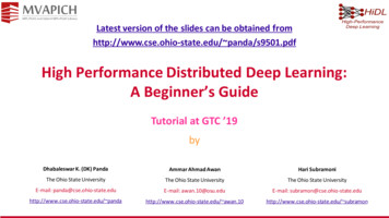
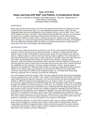
2) Gradient staleness: As the frequency of parameterupdates grows, it becomes increasingly likely that a gradientreceived by the server was computed using a significantlyoutdated model. This increases the noise in the parameterupdates and could potentially slow down the optimizationprocess and lead to problems with convergence. In practice,using adaptive learning rate methods like RMSprop or AdaGrad, we do not see such issues. However, as the number ofworkers increases, this could become a significant problemand should be examined carefully.V. N UMERICAL E XPERIMENTSTo validate our approach, we apply it on the classic gameof Snake and empirically demonstrate the performance ofour algorithm.A. SnakeWe implemented the Snake game in Python and preprocessthe frames of the game to feed in to our neural network(see Fig. 2). In the DistBelief implementation, each workerspawns its own game instance and generates experiencebased on its current model. The game is made up of a n narray with hard walls. The snake starts with body length oftwo and gains an additional body length when it eats anapple. At game termination, due to the snake hitting itselfor one of the walls, the agent loses one point. The goal ofthe game is to maximize the score, equal to the apples eatenminus one. Each worker sends their model to the server afterevery gradient computation, and receives the latest modelfrom the server periodically as detailed in Section IV.E. Implementation detailsAll code for this project can be found, together withdocumentation, e rely on a slighted out-of-date version of Caffe (whichis included as a submodule) as well as Spark for runningthe multi-worker version of distributed deep Q-learning. Ourimplementation does not make heavy use of Spark. However, Spark does facilitate scheduling of gradient updates,coordinating the addresses of all machines involved in thecomputation, and shipping the necessary files and serializedcode to all of the worker nodes. We also made some progresstowards a more generic interface between Caffe and Sparkusing MemoryDataLayers and shared memory. For this,please see the shmem branch of the GitHub repository.rawscreendownsample grayscalefinalinputF. Complexity analysis1) Convolutional neural network: To analyze our modelcomplexity, we break our neural network into three components. The first part consists of the convolutional layersof the convolutional neural network (CNN). The complexityfor this part is O d 2 F k 2 N 2 LC , where we have framewidth d , frame count F , filter width k, filter count N ,convolution layer count LC . The second part consists of the fully connected layers and its complexity is O H 2 LB ,where H is the node count and LB is the hidden layercount. Finally, the “bridge” between the convolutional layers and fully connected layers contributes a complexity ofO Hd 2 N . The total number of parameters in the modelp is thus O d 2 F k 2 N 2 LC C H 2 LB C Hd 2 N . We use thevariable p to simplify our notation.2) Runtime: Consider a single worker and its interactionwith the parameter server. The run-time for a single parameter update is the time to compute a gradient, T , plus thetime to perform the update, . Both T and are O.p/, butthe constant factor differs substantially. Further, the servertakes at least time to perform an update, regardless of thenumber of workers.Thus the run-time for N parameter updates using k workermachines is O .Np k/ if k T or O.N / otherwise.3) Communication cost: Each iteration requires both amodel and a gradient to be sent over the network. Thisis O.p/ data. We do this for N iterations. Thus the totalcommunication cost is O.Np/.Fig. 2: Preprocessing consists of downsampling and grayscaling the image, and an optional step that crops the imageto the input size of our neural network.B. Computation and communicationFigure 3 shows the experiment runtimes with differentmodel sizes, which correspond to different game frame sizes.The legend is as follows. “comms” refers to the amountof time required for sending the model parameters between(either way) the parameter server and one worker. “gradient”refers to the compute time required to calculate a gradientupdate by a worker. “latency” refers to the amount of timerequired by the parameter server to update its weights withone set of gradients. The training rate was compute-boundby gradient calculations by each worker in our experiments.Note that the gradient calculation line is two orders ofmagnitude larger than the other two lines in the figure. Notealso that the upper bound on number of updates per secondis inversely proportional to number of parameters in themodel, since the single parameter server cannot update itsweights faster than a linear rate with respect to the numberof updates in a serial fashion. Thus as the number of workersand model size increase, the update latency might become the5
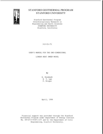
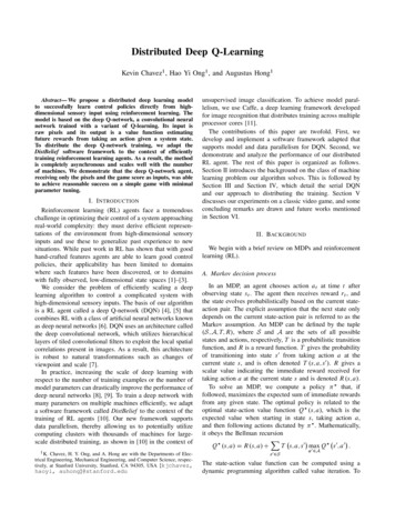
bottleneck of the learning process. To alleviate such a case,we can increase the minibatch size for each gradient update.This modification would therefore increase the compute timerequired by each worker machine and therefore reduce therate at which gradient updates are sent to the parameterserver. Additionally, the gradient estimates would be betterdue to the larger minibatch size.experimental times1average reward150serialdoublecomms (x1 ms)gradient (x100 ms)latency (x1 ms)01100050100200300wall clock time (min)Fig. 4: Comparison of average reward increase betweenthe serial and distributed implementations. The distributedimplementation used two workers.00246number of parametersworker machines will strongly impact model convergencerates.8 106R EFERENCESFig. 3: Compute and communication times for various processes.[1] G. Tesauro, “Temporal difference learning and TDGammon”, 1995.[2] M. Riedmiller, T. Gabel, R. Hafner, and S. Lange,“Reinforcement learning for robot soccer”, Autonomous Robots, vol. 27, no. 1, pp. 55–73, 2009.[3] C. Diuk, A. Cohen, and M. L. Littman, “Anobject-oriented representation for efficient reinforcement learning”, in Proceedings of the 25th international conference on Machine learning, ACM, 2008,pp. 240–247.[4] V. Mnih, K. Kavukcuoglu, D. Silver, A. Graves, I.Antonoglou, D. Wierstra, and M. Riedmiller, “Playing Atari with deep reinforcement learning”, arXivpreprint arXiv:1312.5602, 2013.[5] V. Mnih, K. Kavukcuoglu, D. Silver, A. A. Rusu, J.Veness, M. G. Bellemare, A. Graves, M. Riedmiller,A. K. Fidjeland, G. Ostrovski, et al., “Human-levelcontrol through deep reinforcement learning”, Nature,vol. 518, no. 7540, pp. 529–533, 2015.[6] J. L. McClelland, D. E. Rumelhart, et al., “Parallel distributed processing”, Explorations in the microstructure of cognition, vol. 2, pp. 216–271, 1986.[7] Y. LeCun, L. Bottou, Y. Bengio, and P. Haffner,“Gradient-based learning applied to document recognition”, Proceedings of the IEEE, vol. 86, no. 11,pp. 2278–2324, 1998.[8] A. Coates, A. Y. Ng, and H. Lee, “An analysis ofsingle-layer networks in unsupervised feature learning”, in International Conference on Artificial Intelligence and Statistics, 2011, pp. 215–223.C. Distributed PerformanceTo validate our theory we collected results from twoexperiments, which were ran for a total of 120,000 gradientupdates. The first experiment was performed using a serialimplementation as documented in [4], [5]. The second experiment was ran with two workers for the same numberof updates. As shown in Fig. 4, the two workers modelexperienced a much faster learning rate than the singleworker model. The performance indicated by the averagereward over time scales linearly with number of workers.Here, the average reward value is the number of apples thatthe snake ate minus one for game termination. At every timestamp, we see that the average reward obtained by the twoworker experiment is roughly twice of the single workerexperiment. This trend suggests that the performance of ourdistributed algorithm scales linearly for the initial trainingphase (until some convergence at some point in time).VI. C ONCLUSION AND F UTURE W ORKWe have developed a distributed deep Q-learning algorithm that can efficiently train an complicated RL agenton multiple machines in a cluster. The algorithm combinesthe sequential deep Q-learning algorithm developed in [4],[5] with DistBelief [10], accelerating the training processvia asynchronous gradient updates from multiple machines.Future work will include experiments with a wider varietyof video games and larger clusters to study the generalizingability and scalability of the method. Such experiments willreveal if issues such as model staleness from having many6
[9] J. Ngiam, A. Coates, A. Lahiri, B. Prochnow, Q. V. Le,and A. Y. Ng, “On optimization methods for deeplearning”, in Proceedings of the 28th InternationalConference on Machine Learning (ICML-11), 2011,pp. 265–272.[10] J. Dean, G. Corrado, R. Monga, K. Chen, M. Devin,M. Mao, A. Senior, P. Tucker, K. Yang, Q. V. Le,et al., “Large scale distributed deep networks”, inAdvances in Neural Information Processing Systems,2012, pp. 1223–1231.[11] Y. Jia, E. Shelhamer, J. Donahue, S. Karayev, J.Long, R. Girshick, S. Guadarrama, and T. Darrell,“Caffe: Convolutional architecture for fast feature embedding”, arXiv preprint arXiv:1408.5093, 2014.[12] M. Hausknecht, J. Lehman, R. Miikkulainen, and P.Stone, “A neuroevolution approach to general atarigame playing”, 2013.[13] K. Jarrett, K. Kavukcuoglu, M Ranzato, and Y. LeCun,“What is the best multi-stage architecture for objectrecognition?”, in Computer Vision, 2009 IEEE 12thInternational Conference on, IEEE, 2009, pp. 2146–2153.[14] D. Precup, R. S. Sutton, and S. Dasgupta, “Off-policytemporal-difference learning with function approximation”, in ICML, Citeseer, 2001, pp. 417–424.[15] J. N. Tsitsiklis and B. Van Roy, “An analysis oftemporal-difference learning with function approximation”, Automatic Control, IEEE Transactions on, vol.42, no. 5, pp. 674–690, 1997.[16] A. W. Moore and C. G. Atkeson, “Prioritized sweeping: reinforcement learning with less data and lesstime”, Machine Learning, vol. 13, no. 1, pp. 103–130,1993.A PPENDIXA. Network architectureFigure 5 graphically visualizes the exact architecture ofour deep neural network, as implemented in Caffe.7
Fig. 5: Deep neural network architecture for numerical experiments.8
Distributed Deep Q-Learning Kevin Chavez 1, Hao Yi Ong , and Augustus Hong Abstract—We propose a distributed deep learning model to successfully learn control policies directly from high-dimensional sensory input using reinforcement learning. The model is based on the deep Q-network, a convolutional neural network trained with a variant of Q .