Transcription
STANFORD GEOTHERMAL PROGRAMSTANFORD UNIVERSITYStanford Geothermal ProgramInterdisciplinary Research inEngineering and Earth SciencesSTANFORD UNIVERSITYStanford, CaliforniaSGP-TR- 7 5USER'S MANUAL FOR THE ONE-DIMENSIONALLINEAR HEAT SWEEP MODELA. HunsbedtS. T. LamP. KrugerApril, 1984Financial support was provided through the StanfordGeothermal Program under Department of Energy ContractNo. DE-AT03-80SF11459 and by the Department of CivilEngineering, Stanford University.
ABSTRACTThis manual describes a 1-D linear heat sweep model for estimating energyrecovery from fractured geothermal reservoirs based on early estimates of thegeological description and heat transfer properties of the formation.Themanual describes the mathematical basis for the heat sweep model and its w eis illustrated with the analysis of a controlled experiment conducted in theStanford Geothermal Program's large physical model of a fractured-rock hydrothermal reservoir.The experiment, involving known geometry and heat transferproperties, allows evaluation of the model's capabilities, accuracy, and limitations.The manual also presents an analysis of a hypothetical field problemto illustrate the applicability of the model for making early estimates ofenergy extraction potential in newly developing geothermal fields.Further development of the model is underway.from one-dimensional linear sweeptoEnhancement of the modalone-dimensional radial sweep will expafidits application for early estimate of energy extraction to more complex geothermal fields.Other improvements to the model may involve inclusion Qfvariable water production/recharge rate and more detailed estimate of the he&transfer from the surrounding rock formation.these enhancements are achieved.iiThe manual will be revised 8s
TABLE OF CONTENTS.iiList of Figures . . . . . . . . . . . . . . . . . . . . . . . . . . . . .iiiList of Tables . . . . . . . . . . . . . . . . . . . . . . . . . . . . . .iv1. Introduction . . . . . . . . . . . . . . . . . . . . . . . . . . . . .12 . Mathematical Model . . . . . . . . . . . . . . . . . . . . . . . . . .42.1Geometry and Assumptions . . . . . . . . . . . . . . . . . . . .42.2 Governing Equations . . . . . . . . . . . . . . . . . . . . . .62.3 Solution Procedure . . . . . . . . . . . . . . . . . . . . . . .9122.4 Definition of Parameters . . . . . . . . . . . . . . . . . . . .Effective Rock Block Radius . . . . . . . . . . . . . . . 132.4.1Energy Extraction Parameters . . . . . . . . . . . . . . 172.4.23 . Sample Problem Analysis . . . . . . . . . . . . . . . . . . . . . . .193.1 Experimental System Problem . . . . . . . . . . . . . . . . . . 193.1.1Physical Model . . . . . . . . . . . . . . . . . . . . .19Input Data Preparation . . . . . . . . . . . . . . . . . 233.1.2Running the Program . . . . . . . . . . . . . . . . . . . 313.1.33.1.4Results . . . . . . . . . . . . . . . . . . . . . . . . .353.1.5Parametric Evaluation of Solution . . . . . . . . . . . . b93.2 Hypothetical Field Problem . . . . . . . . . . . . . . . . . . . 613.2.1Problem Description . . . . . . . . . . . . . . . . . . . 413.2.2Results . . . . . . . . . . . . . . . . . . . . . . . . .66I4 . Nomenclature . . . . . . . . . . . . . . . . . . . . . . . . . . . . .545 . References . . . . . . . . . . . . . . . . . . . . . . . . . . . . . .56AbstractAppendices.B.Flow Diagram for l-D Linear Heat Sweep Model Program . . . . . .C . Experimental System Problem Output . . . . . . . . . . . . . . .Al-D Linear Heat Sweep Model Program Listing576061
LIST OF FIGURESFigure2- 13-13-23-33-43-53-63-73-8Page.Experimental Rock Matrix Configurationand Thermocouple Locations . . . . . . . . . . . . . . .Probability Rock Size Distribution for Regular ShapeRock Loading used in Experiment 5-2 . . . . . . . . . . .Comparison of Measured and Predicted Water Temperaturesfor Experiment 5-2 . . . . . . . . . . . . . . . . . . .l-D Linear Heat Sweep Model GeometryEnergy Extracted Fraction, Energy Recovery Fraction,and Produced Water Temperature as Functions ofNon-dimensional Time for Experiment 5-2.Effect of Number of Terms in the Laplace InversionAlgorithm on the 1-11 Model Prediction . . . . . . . . . .Probability Rock Size Distribution for HypotheticalFieldproblem.3-103-1 120218363184104bPredicted Water and Rock Temperatures for HypotheticalField Problem--Ntu 51.84)Energy Extracted Fraction, Energy Recovery Fraction,and Produced Water Temperature as Functions ofTime for Hypothetical Field Problem--Ntu 51.848Predicted Water and Rock Temperatures for HypotheticalField Problem--NtU3.25P.3-95.Energy Extracted Fraction, Energy Recovery Fraction,and Produced Water Temperature as Functions ofTime for Hypothetical Field Problem--Ntu 3.2sComparison of Calculated Water and Rock Temperature atX* 0 from Analytical Solution and Solution Obtainedby Numerical Inversion.iii5P53
LI:STOF TABLESPageTable1-11-22-13- 13- 23-33- 43- 53-63-73- 8.Results of Early Heat Extraction Experiments . . . . . . .Coefficients for Inversion of the Laplace Transform . . . .Experimental Data and Parameters for Experiment 5-2 . . . .Time-Temperature Data for SGP Physical ModelExperiment 5-2 . . . . . . . . . . . . . . . . . . . . .List of Experimental Parameters to Linear Heat Sweep Modelfor SGP Physical Model Experiment 5- 2 . . . . . . . . . .Calculation of Sums for Effective Rock Size Calculation.Experimental System . . . . . . . . . . . . . . . . . . .Hypothetical Field Problem Data . . . . . . . . . . . . . .Hypothetical Field Rock Size Data . . . . . . . . . . . . .Calculation of Sums for Effective Rock Size Calculation.Hypothetical Field I?roblem . . . . . . . . . . . . . . .Summary of Input Parameters to Linear Heat Sweep Model forHypothetical Field I?roblem . . . . . . . . . . . . . .Relative Recovery froin Hydrothermal Reservoirsiv331221223214219&/24144446
1.INTRODUCTIONSince 1972, the Stanford Geothermal Program has had a continuous objec-tive of investigating means of enhanced energy recovery from geothermalresources.One of the key objectives is the technical basis for early assess-ment of the amount of extractable energy from hydrothermal resources underThe l-D Linear Heat Sweep Model has beenvarious production strategies,developed from a physical model oftifractured rock, hydrothermal reservoir toestimate the potential for energy extraction based on limited amounts ohgeologic and thermodynamic data.The potential for energy recovery from hydrothermal reservoirs was exam ined by Ramey, Kruger, and Raghavan (1973) for hypothetical steam and hotwater reservoirs similar in size arid properties.The data in Table 1-1 werecalculated for geothermal reservoirs at an initial temperature of 260 C,porosity of 25 percent over a reservoir volume 1230 m3 in extent, with steahenthalpy of 2.33 MJ/kg for a useful life based on pressure decline from 4.5MPa (at 260OC) to an abandonment pressure of 0.7 MPa (at 164OC).The datbshow that only 6 percent of the available energy in the steam reservoir is it the geofluid, while 94 percent is in the formation rock.It is apparent thata method of "sweeping" the heat i.n the rock by recycling of cooler waterthrough the reservoir could signific:antly enhance energy recovery.The development of the l-D Linear Heat Sweep Model has been accomplishedi n three phases.The first phase! involved a lumped-parameter analysis ofenergy recovery using three non-isothermal production methods (Hunsbedt,Kruger, and London, 1978):(2)(1) pressurereduction within-place boiling;reservoir sweep with injection of cold water; and (3) steam drive withpressurized fluid production.Table 1-2.Results of these studies are summarized ilhFrom a thermodynamic point of view, it appears that reservoit
sweep with cycled cold water (under carefully controlled conditions to avoidshort-circuiting and mineral deposition) could effectively enhance overallenergy extraction.The second phase involved development of a heat transfer model for acollection of irregular-shaped roc:ks with arbitrary size distribution.THeefforts of Kuo, Wuger, and Brigham (1976) resulted in adequate correlatiodsof shape factors with thermodynamic properties of single irregular-shaped roQkThe work by Iregui, Hunsbedt, Kruger, and London (1979) extended theblocks.correlations to assemblies of fractured blocks.The result was a on -dimensional model of a hydrothermal, fractured rock system under cold watdrinjection heat sweep based on a single spherical rock block of "effectiqeradius".The third phase of the development has been based on experimental verifllcation of the ability of a l- D heat sweep model to predict energy recoventyfrom a rock loading of known, regular geometric shape and thermal properties,The model is based on input knowledge of the volumetric distribution of rodkblocks and the rock heat transfer parameters.The experimental parameters afthe model are the "number of heat transfer units" and the initial distributianof energy stored in the water and rock.The "number of heat transfer units"parameter is determined by the estimated fluid residence time and the tiaeconstant for the rock block (a function of equivalent rock radius, therm&diffusivity, and Biot number).As the most significant parameter in the 1 4Heat Sweep Model, it indicates thie degree to which energy extraction fromupotential hydrothermal reservoirs is heat transfer limited or water supplvlimited.This manual describes the mathematical basis for the model and provides aworking means for its use through analysis of two sample problems.2The model
---u1is intended for early use in analysis of new geothermal reservoirs to testevaluations of geologic estimations of rock type and fracture distribution.Early application of the model to real reservoirs should provide feedback asto current model limitations and a basis for improvements.Further developi-ment of the model is expected to enhance its applicability in the earxyanalyses of more complex geothermal reservoirs.Table 1-1RELATIVE RECOVERY FROM HYDROTHERMAL RESERVOIRS*Steam ReservoirFluid- RockHot Water ReservoirRockFluid7,330242,10088528,260Production (kg)6,445213,840as Steam6,445168,740as Water045,1001610687.988.36.199.1Reservoir Mass (kg)Abandonment Content (kg)Available Energy (GJ)Recovery of Fluid Mass ( X )Recovery of Available Energy*for a hypothetical reservoir of 26OOC temperature, 25% porosity,123Om3 volume, 2 . 3 3 MJ/kg steam enthalpy, and abandonment pressureof 0.69 MPa (at 164OC). Adapted from Ramey, Kruger, Raghavan ( 1 9 7 3 ) .Table 1-2RESULTS OF EARLY HEAT EXTRACTION EXPERIMENTSProductionMethodIn-Place BoilingSweepSteam DriveSpecific EnergyExtraction (kJ/kg)83145-Energy ExtractionFraction ( X )11675-17580-10086*22-2721*Based on steady-state water injection temperature. Othersbased on saturation temperature at final pressure. Adaptedfrom Hunsbedt, Kruger, and London, (1977).3
2.MATHEMATICAL MODELThe one-dimensional linear sweep model is designed to calculate water androck matrix temperature distributions in a fractured hydrothermal reservoir asfunctions of distance from the injection point and time of production.2.1Geometry and AssumptionsThereservoir geometry ofB.1-Dheatsweep modelis given ihCold water at temperature Tin is injected through a line of well Figure 2-1.at pointtheAand produced at the same rate through a line of wells at pointThe distance between the injection and production wells iscross-sectional area of the reservoir isS.L,and theThe initial temperature of boththe reservoir water and rock is TI everywhere in the reservoir.The colb1water injection temperature Tin may be constant or decrease exponentially fro@the initial reservoir temperature to a lower constant value.The reservoir rock consists of rock blocks of various sizes and ofirregular shape.The intrinsic permeability of the rock blocks is essentiallyIzero while the permeability of the reservoir is considered to be essentialliinfinite.Based on the work of Kuo et al. (1976),it is assumed that the rockformation is thermally characterized by a single effective block size ofradius Re,c.reservoir.The rock block size distribution is assumed to be uniform in theThe fracture porosity and flow velocity in the reservoir arqassumed to be constant over the cross-sectional area (S), and do not vary witbdistance (L) between the injection and production wells.Heat transfer per unit reservoir length and per unit time q 'along thkdirection of flow is assumed to be constant in time and space.The signconvention used is thatq'is positive when heat flow is from the surround?ing rock formation to the reservoir rock formation.4Two-dimensional effect
mPmiSFig. 2-1:1-D Linear Heat Sweep Model Geometry15
such as gravity segregation of cold water to the bottom layers of thereservoir, and axial heat conduct:Lon are neglected.Physical and thermalproperties of both water and rock are assumed to be constant.The 1-D heat sweep model takes into account the temperature gradienltinside large rock fragments produced by long path lengths for heat conductionand low rock thermal conductivity when cold water flows along the rock surfaces.Previous analyses performed by Schuman (1929) and L6f and Hawlep(1948) for air flowing through a rock matrix neglected the thermal resistanceIinside the rock itself while considering only the surface resistance.assumption may be correct for air flow.ThibIt is not acceptable for waterbecause the surface resistance is usually very low compared to the internakrock thermal resistance, indicated by a high Biot number.2.2Governing EquationsIA thin element of the reservoir (shown in Figure 2-1) of thicknessand cross-sectional areaSdkis the representative volume in deriving thkgoverning equation for the reservoir water temperature.AnPenergy balance othis element results in the following partial differential equation for thkwater temperatureThe initial and boundary conditions, respectively, areTf(O,t) (T -T )e Bt1 in 6Tin(2-lc)
Explanation of the symbols used in the manual are compiled in the nomenclaturesection.The parameterB, referredto as the recharge temperature parame-ter is selected by the user to give the desired inlet condition.it is noted that BEq. (2-lc), -ODhr-'gives a step change in the waterinlet temperature while a finite and negative value oftially decreasing inlet temperature.Referring tr,Bgives an exponea-For well defined situations, such asflow of recharge water down an injection well, it is possible to estimate thevalue ofBusing the procedure developed by Ramey (1962).In other cases,however, the flow path of surface water recharge in a geothermal reservoir maybe undefined, and B -ODhr"is recommended whenBcannot be estimated.An energy balance on the rock fragments within the differential elementgives for the average rock temperatureaTr- atThe conduction path length lcond is used to represent the internal rock thettmal resistance.The ratio lcond/Rck,cwas determined to be approximately 0.for spherical shapes (Hunsbedt et al. (1977) and Iregui et al. (1979)).time constant for the rock fragments of radius Re,c is defined ashTheIR 2(2-2b)T Reference is made to section 2.4.1for definition of Re,c, referred to as theeffective rock size of a rock collection.Eq. (2-2a) gives for the rock temperature7Substituting the time constant into
T -Tf r-aTr -at(2-2c)fwhich is solved with the initial conditionEquations (2-la) and (2-2c) are a set of coupled partial differentialequations, which can be simplified by introducing non-dimensional variables agfollows:Temperature:(2-3aD(2-3b)Space :x* x/L(2-34Time :t* t/tre(2-3d)Number of Heat Transfer Units Parameter:NtuEtre/r(2-3e)External Heat Transfer Parameterq* q'L/PufSCf(T1-Tfn)l(2-3f)Storage RatioY PfCf /PrCr(1- )(2-3g)Recharge Temperature ParameterB* Bt,,(2-3h)8
.- -These non-dimensional variables and parameters allow the partial differentialequations and boundarylinitial conditions to be written asaT*aTf* aTf* -- ax*at*Y at*( 2-4a)q**Tf ( " 0 )1(2-4b)Tf* (O,t*) eB * t *(2-4 )and(2-4d)-Tr*2.3(2-4eb(x*,O) 1Solution Procedure1IAnanalytical solution to the governing equations is not availabletHowever, a solution has been obtained by numerical integration using finitedifference techniques.The technique adopted for the model involves transfor-ming into the Laplace space combined with a numerical inversion algorithm.The Laplace transform of Eqs. (:2-4a), (2-4c), and (2-4d) with the initia!.conditions given by Eqs. (2-4b) and (2-4e) results in the following set ofequationsAAAaTf* s Tf*ax*1- 1 -Y [ S Tr**sTr*-1 NtU ( Tf*-with boundary condition9-Tr*)11 q*/S(2-5ab(2-5bb
A-*Tf (0,s) l/(sB*:)(2-5 )AEquations (2-5a) and (2-5b) can be solved for*Tf andTr*togive for thewater temperaturendTf*dx* Ksif K(2-6a)Ntu NtJ(2-6b)whereK 1 Y(SIntegration of Eq. (2-6a) using condition (2-5c) gives the water temperatureasTf"* (3 -)1SKs- - - -11 (-- 1Q*S-B*e-Ksx*(2-7a)Ks2The corresponding Laplace equation f o r the rock temperature isA- * -Tr N -1sNtU ANt:u(2-7b)Tf*Inversion back to real time space gives as the fluid temperatureTf*(x*, t*) x-' [ Tf*(x*, s 1Inversion ofthe Laplace transform is performedalgorithm given by Stehfest (1970):10(2-8)numerically usingthe
-1 1I,*Tf (x*,t*)In 2 -t*Mci ll ai Tf (x*,It*n 2xi)A*(2-9a)where the coefficients are given byMinai (-1)M/ 2 i(i ,,M/2)ck(M/2)( 2k) !Mi l(k (-F)2The coefficients are independent of time,terms, M-k)!k!(k-l)!(i-k)!(2k-i)!(2-9b)sothat once the optimum number of, has been selected, one computation of the coefficients is suffitcient for all times.magnitudes ofyThe value ofMchosen largely depends on the, Ntu, and computer accuracy.determine the optimum value ofMResults of a study t bare presented in section 3.1.5.It wagfound that, in general, values between 8 and 14 produced good practicalresults, and that a problem with a higherhigher number of terms.between 4 and 12.Ntuvalue usually requires aTable 2-1 shows these coefficients for values ofThe Stehfest algorithm solution to Eqs. (2-7a) and (2-7b)can readily be programmed on a hand calculator or microcomputer.A program tbperform the calculation is given in Appendix A and a flow diagram of theprogram in Appendix B.Use of the solution will be demonstrated in late sections.11
Table 2-1COEFFICIENTS FOR INVERSION OF THE LAPLACE TRANSFORMCoefficients ai for given -0.01666.16.0166. .-12471279. 84,244.166. 7-212359,251 - 2*. means that the figures continue infinitely.Recommended for optimum solutions: M 8 or 102.41(M must be an even number).tDefinition of ParametersThe prediction of energy extrac:tion from a fractured geothermal reservoirrequires a mathematical heat transfer model to estimate the average rocktemperature relative to that of t:he surrounding fluid.It also requiresinformation on the rock size and shape distributions which are difficult todetermine for real geothermal reservoirs.The rock heat transfer model usedin the linear heat sweep model was therefore developed in section 2.4.112for
general size and shape distributions.Evaluation of energy extraction for avariety of assumed reservoir rock parameters can thus be carried out in earlystages in the development of a geothermal resource.2.4.1.Effective Rock Block RadiusThe rock heat transfer model was first developed from the work of Kuo,Kruger, and Brigham (1976) for a single rock block of irregular shape byintroducing the concepts of a sphericity parameter and effective heat-transferradius.These concepts were derived on the premise that the thermal behaviorof an irregularly shaped body can be approximated as a spherical body havingthe same surface area to volume ratio.The Kuo sphericity parameter isdefined bywhereAs 411Rs2 surface area of a spherical rock with thesame volume as the irregularly shaped rockAactual actual surface area of the rock block(2-lob)radius of a sphere with the samevolume! (v) as the irregularly shapedro c:k b1o ck(2-1041/3RS [ I3v The sphericity is less than unity for all geometric shapes other than thesphere.Equation (2-loa) implies t.hat there is an "effective" sphere radiuswhich will give the correct thermal response for an irregularly shaped rockblock.The investigation, carried cut by Kuo, Kruger, and Brigham (1976) on avariety of regular and irregularly shaped bodies, showed that such an effective radius could be approximated by13
Re YK(2-11)x RsThe investigation also showed that surface area to volume ratio is not theonly parameter that determines heat: transfer from irregularly shaped bodies,It was expected that a "form factor" which characterizes the effective conduetion path length would also have some influence particularly for block shapeswhere one dimension is much small-er than the other two.neglected in the linear sweep heat model.This effect i sIn some cases it is possible toapproximate the rock blocks shape as flat plates.The theoretical basis forthis approach will be considered for inclusion in later versions of thi6manual.The heat transfer model for a collection of unequal size rock blocks isbased on the earlier observation that the surface area to volume ratio of 8single rock was the main parameter governing the heat transfer.ratioiscalculatedforthecollection ofrocks withaWhen thisgivensiaedistribution, an "effective" single spherical rock having equal surface aresto volume ratio may be used in the heat transfer prediction.The surface area to volume ratio for the collection is derived usin Eqs. (2-10) and (2- 11) for each blocki in the size distribution and summing;Ifor all blocks Nasi 1It is more efficient in the numerical calculation of these sums to considarseveral size groupsNLeach containing approximately equal size block 14
rather than each block individually.bility density functionP(R,, )size rock blocks in thejth group.This is done by introducing the proba- nj/Nwherenjis the number of equalThe equivalent size sphere that has thiesurface area to volume ratio is determined from the ratiowith radius R.3/Rfor a sphereHence, the equivalent size sphere radius, referred to as the"effective radius" for the collection is defined by-R YKe,c(2-123j lwhere-YK is the average sphericity.The effective radius used in the heat transfer calculation can be thoughtof as being the "thermal center" for the collection of rock blocks.greater than the mean radiusRswhereas with-% /Rs -/z0-R isand it is skewed by dispersion about themean toward the larger-sized rock blocks.tion with a value ofIt0.3,For example, for a normal distribuRe,cis 20 percent higher than-RsS1, Re,c is 111 percent higher.SMeasurements were carried out for the size distribution of a rock samplefrom the Piledriver granitic rock chimney* consisting of 360 rock blocks an4on six "instrumented blocks" with t'hermocouples embedded at the block centers[Iregui et al. (1979)l-to determine a typical average value of the sphericitjlY K for use in Eq. (2-12).The mass, length, breadth, and width (approximateorthogonal axes of the rock) were measured for each block.In addition, thesurface area of the six instrumented blocks were determined by a paraffincoating technique used by Kuo, Kruger, and Brigham (1976).*The Piledriver (61-kt) nuclear explosive was detonated on June 2, 1966 at adepth of 1,500 ft (457m) in a granodiorite formation.15
Since it was not practical to measure the surface area of all blocks inthe sample, an approximate method of obtaining surface area was found in whichthe actual area was computed assuming the block shape is an ellipsoid with thkmeasured length, breadth, and width as axes.1'VK,red to as the pseudo sphericityblocks for which the Kuo sphericity YKThe resulting sphericity, refer-was compared for the six instrumented[Eq. (2-10a)l based on an independentsurface area measurement using the paraffin-coating technique was available.The comparison showed thatblocks.IYgwas within 10 percent ofYKfor these rockThe average ratio between the two was found to beyKT 0.97 f 0.06(2-13)yKwith a 95 percent confidence level.The pseudo sphericity was plotted as a function of rock block size.Thescatter in the data was found to be significant and a least-squares regressionanalysis was carried out to determine if a trend in the data could be estabrlished.The linear equation representing the "best fit" isY K (0.838 0.005 R,,) & 0.16(2-14)L)A coefficient of determination of 0.0195 shows that only 1.95 percent of thevariation in1YKis explained by variation in block size, i.e., the spheric-ity is practically independent of block size for the collection considered,This finding was reinforced by noting that the probability distributions of1YKand the two ratios of measured block axes were found [Isegui et alc(1979)lto be well represented by normal distributions.It is thereforeassumed that the sphericity of this rock collection can be represented by a16
mean value obtained from Eq. (2-14) and corrected by Eq. (2-13) to give a meansphericity of-YK (2-15)0.97 x 0.86 0.83-Y is adopted in th!e linear heat sweep model for irregularlyKshaped rock blocks found in geothermal reservoirs.This value of2.4.2Energy Extraction ParametersParameters used in assessing the degree of energy extraction from thkreservoir are defined and calculated by the program listed in Appendix A.Ameasure of the degree of energy ex:traction from a rock distribution at timetis defined by(2-16)This fraction is referred to as the "energy extracted fraction" and measure6the amount of energy actually extracted when the rock is cooled from theinitial temperatureT1to the average temperatureTrrelative to thatextracted if the rock is cooled to the surrounding fluid temperature Tf.The "temperature drop fraction" for the reservoir is calculated from i C definition asT1Fc TI- Tf 1 - TinIo1*Tf(x*,t*)dx*(2-17)The temperature drop fraction is a measure of the average reservoir watertemperature relative to the injection water temperature at time t.17
A measure of total energy extracted at timetto thermal energy storedin rock and water, denoted by the “energy recovery fraction,“ is given bylz*Tf* ( 1 , t*)dt*F 1P (2-181)l/yFinally, the energy extracted fraction for the whole reservoir, asdefined earlier for a single rock block (Eq. 2-16) is calculated for a rockblock distribution in terms of the two previous parameters for negligibleexternal heat transfer as(2-19)This parameter is a measure of average rock temperature relative to averagewater temperature at timerock and water.t,i,,e., degree of thermal equilibrium betweenFor example, FE,c 1 implies complete thermal equilibriua,From Eq. (2- 19) it can be seen that the energy recovery fraction for a lowporosity (A 5%) reservoir (in whic’h ythe product ofFE,c andFp FE,cFcapproaches zero) is proportional t o, or(2-20)FcEquation (2- 20) shows that energy recovery from a fractured reservoir can belimited by a smallFE,c(heat transfer limitation possibly because of vervlarge rock blocks) or by a smallF,which can occur, for example, if thewater flows along preferred paths (fingering effect) in which regions of thereservoir have high water temperatures and correspondingly low rock to watertemperature differences to affect the heat transfer from the rock blocks.18
3.SAMPLE PROBLEM ANALYSISThe application of the 1-D linear heat sweep model is illustrated withtwo sample problem analyses.The first one is the analysis of an experimenltperformed in the Physical Reservoir Model of the Stanford Geothermal Programand the second problem is a hypothetical field case study.These two problemsillustrate the preparation of input data and the interpretation of programoutput.3.1-Experimental System ProblemThe application of the linear heat sweep model to the physical modelexperiment illustrates input preparation, interpretation of output data,accuracy of model prediction relative to experimental results, and the basisfor choosing the optimum number of t:erms in the Stehfest algorithm for numericcal inversion ofthe Laplace Transform.Abriefdescription oftheexperimental system is presented as an aid in interpreting the results.3.1.1Physical Model of a Frac:tured Hydrothermal ReservoirThe SGP physical model has been described in several reports, e.g.,Hunsbedt, Kruger and London (1975, 1977, 1978).The main component is 81.52 m (5 ft) high by 0.61 m (2 ft) diameter insulated pressure vessel.Therock matrix in the reservoir model consists of 30 granite rock blocks of 0.19x 0.19 m (7.5 x 7.5 inches) square cross section and 24 triangular blocks asshown in Figure 3-1.The blocks are 0.26 m (10.4 inches) high.The averagltfracture porosity of the reservoir is 17.3 percent.Vertical channels between blocks are spaced at 0.64 cm (0.25 inch) andhorizontal channels between layers are spaced at 0.43 cm (0.17 inch).Signif icant vertical flow can occur in the relatively large edge channels betweehthe outer rock blocks and the pressure vessel walls.19
Sy mbo I Description0AV0WaterRockWaterMetalQ iuant it y246INFig. 3-1:Experimental Rock Matrix Configuration and Thermocouple Locations20
Cold water is injected at the bottom of the vessel by a high pressurepump through a flow distribution baffle at the inlet to the rock matrix.System pressure is maintained above saturation throughout the production runby a flow control valve downstream of the vessel outlet.The rock blocks haveessentially zero permeability while! the flow in the spaces between the rockblocks is characterized by essentially infinite permeability.Most of thesystem pre
STANFORD UNIVERSITY Stanford, California SGP-TR- 7 5 USER'S MANUAL FOR THE ONE-DIMENSIONAL LINEAR HEAT SWEEP MODEL A. Hunsbedt S. T. Lam P. Kruger April, 1984 Financial support was provided through the Stanford Geothermal Program under Department of Energy Contract No. DE-AT03-80SF11459 and by the Department of Civil Engineering, Stanford .