Transcription
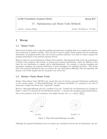
10-708: Probabilistic Graphical ModelsSpring 201717 : Optimization and Monte Carlo MethodsLecturer: Avinava Dubey11.1Scribes: Neil Spencer, YJ ChoeRecapMonte CarloMonte Carlo methods such as rejection sampling and importance sampling allow us to compute the expectation of functions of random variables. They can also be used to simply obtain samples from the underlyingdistribution. In graphical models, they can be used to perform inference, even when we cannot compute themarginal distribution or the partition function directly.However, there are several limitations of Monte Carlo methods. One important issue is that the performanceof Monte Carlo methods relies heavily on having good proposal distributions, which are difficult to findwhen the true distribution is complex and/or high-dimensional. For example, in rejection sampling andimportance sampling, the proposal distribution is fixed throughout the sampling procedure. This meansthat if the proposal distribution does not capture the true distribution sufficiently well, the algorithm willpropose a lot of bad samples and the acceptance rate will be low.1.2Markov Chain Monte CarloMarkov Chain Monte Carlo (MCMC) gets around this issue by having a proposal distribution conditionedon the current sample. In Metropolis-Hastings, the acceptance probability of a proposal is the ratio ofimportance weights and favors more “important” samples.However, Metropolis-Hastings also has a problem of its own. Consider the two-dimensional toy example inFigure 1, where P (x) denotes the true distribution and Q(x0 x) denotes the symmetricproposaldistribution.no0)Due to the symmetry of Q, the acceptance rate simply becomes A(x0 , x) min 1, PP(x(x) .xx2x1(b) Q(x0 x)(a) P (x)Figure 1: When Metropolis-Hastings can suffer.Although the proposal distribution does not assume any correlation between the two dimensions, the (un1
217 : Optimization and Monte Carlo Methodsknown) true distribution has a high correlation, as shown in Figure 1. Then, when the current sample isat x1 , where the contour of P is flat (i.e. gradient is small), the proposal distribution Q(x0 x1 ) has arelatively small variance, so it will explore the sample space more slowly – that is, it will display a randomwalk behavior. Conversely, when the current sample is at x2 , where the contour of P is steep (i.e. gradientis large), the same proposal distribution Q(x0 x2 ) will now have a relatively large variance, so that manyproposed samples will be rejected.The two contrasting cases demonstrate that simply adjusting the variance of Q is not enough, because thesame variance can be small in certain regions and large in others. When the variance is too small, the nextsample is too close to the previous one. When the variance is too large, the next sample can more easilyreach a low-density region in P , so it is more easily rejected. Either case leads to a lower effective samplesize and slower convergence to the invariant distribution.How do we get around this issue? One way is to make use of the gradient of P , as suggested above; thisleads to Hamiltonian Monte Carlo (Section 2). Another way is to approximate P directly, for example usingvariational inference, and using the approximation as our proposal distribution (Section 3).2Hamiltonian Monte CarloHamiltonian Monte Carlo, or Hybrid Monte Carlo, is a specialized Markov Chain Monte Carlo procedurewhich unites traditional Markov Chain Monte Carlo with molecular dynamics. It was originally proposedby [1], but [2] is widely credited with introducing it to the statistics and machine learning communities inthe context of performing inference on Bayesian neural networks.For a more thorough explanation of HMC and its variants than is provided here, see the classic survey paper[3], or the more recent[4].2.1Hamiltonian DynamicsBefore introducing HMC, it is necessary to provide some background on the molecular dynamics on whichit is based: Hamiltonian dynamics. Note that it is not essential that one grasps the motivating physics tounderstand the components of the HMC algorithm. However, the basic physical concepts are useful in thatthey provide intuition.The basics of Hamiltonian dynamics are as follows. Consider the physical state of an object. Let q and pdenote the object’s position and momentum, respectively. Note that each of these variables has the samedimension.The Hamiltonian of the object is defined asH(q, p) U (q) K(p)where U is the potential energy and K is the kinetic energy. Hamiltonian dynamics describe the nature bywhich the momentum and position change through time.This movement is governed by the following system of differential equations called Hamilton’s equations: Hdqi dt pidpi H dt qi(1)(2)
17 : Optimization and Monte Carlo Methods3Illustration of the intuition Consider a frictionless puck lying on a surface whose height. Here, considerU (q) as proportional to the height of the surface at position q. Also, let p denote the momentum of thepuck. Let K(p) p2 /2. Figure 2 illustrates the movement of the puck according to Hamiltonian dynamics.(a) The initial placement of the puck(b) Simulation of the Hamiltonian movement of thepuck. The puck continues moving in the direction ofthe green arrow until H(q, p) U (q) and momentumis 0.(c) After reaching maximum U (q), the puck now reverses direction and continues until the same heightis reached in the other direction.Figure 2: An illustration of the intuition of Hamiltonian Dynamics. The puck is shown in black. The surfaceis shown in red and blue, with the blue showcasing an area where the surface is flat. The green representsthe movement of the puck.For a concrete example for which Hamilton’s equations can be solved analytically, consider U (q) q 2 /2.Here, the solutions have the form q(t) r cos(a t) and p(t) r sin(a t) for some a.There are several important properties Hamiltonian dynamics which end up being useful in the context ofHamiltonian Monte Carlo. First, it is reversible, meaning that if the momentum of the body is reversed,it will retrace its previous movement. Also, the Hamiltonian is preserved: as the kinetic/potential energy
417 : Optimization and Monte Carlo Methodsincreases the potential/kinetic energy decreases accordingly. That is, X d d XdHdpi H H Hdqi H H H 0.dtdt qidt pi pi qi qi pii 1i 1where d is the dimension of the space. This can be thought of as “conservation of energy”.Finally, volume is preserved under the mapping by Hamiltonian dynamics (Louisville’s Theorem).2.2Numerically Simulating Hamiltonian DynamicsIn general, it is not possible to analytically solve Hamilton’s equations as we did for the simple case above.Instead, it is common to discretize the simulation of the differential equations with some step size ε.We briefly discuss two options here: Euler’s method (performs poorly) and the leapfrog method (performsbetter).Suppose that the momentum has the following expression (as is typical)K(p) dXp2i2mii 1Euler’s method involves the following updates:dpi(t)dt U pi (t) ε(q(t)) qidqiqi (t ε) qi (t) ε(t)dtpi (t) qi (t) εmipi (t ε) pi (t) εUnfortunately, Euler’s method performs poorly. The result often diverges, meaning that the approximationerror grows causing the Hamiltonian to no longer be preserved. Instead, the leapfrog method is used inpractice.The leapfrog method deals with this issue by only making a ε/2 step in p first, using that to update q, andthen coming back to p for the remaining update. It consists of the following updates: U(q(t)) qipi (t ε/2)qi (t ε) qi (t) εmi Upi (t ε) pi (t ε/2) (ε/2)(q(t ε)) qipi (t ε/2) pi (t) (ε/2)The leapfrog approach diverges far less quickly than Euler’s method. We now have the necessary tools todescribe how to formulate a MCMC strategy using Hamiltonian dynamics.
17 : Optimization and Monte Carlo Methods2.35MCMC using Hamiltonian dynamicsHamiltonian Monte Carlo uses Hamiltonian dynamics to make proposals as part of an MCMC method.To do so, auxiliary “momentum” variables are introduced to create an auxiliary probability distribution asfollows. Note that this auxiliary distribution admits the target distribution as a marginal.Suppose that P (q) π(q)L(q D) denotes our target density (the posterior of q given prior π and data D),with q denoting our variables of interest. Define the auxiliary distributionP (q, p) P (q) exp( K(p))1 exp ( U (q)/T ) exp( K(p))ZwithU (q) log [π(q)L(q D)]K(p) dXp2i2mii 1Note that the auxiliary momentum variables are assumed to be independent gaussians.2.4Sampling AlgorithmWe want to sample from P (q, p). Note that because p is independent of q and has a tractable form (Gaussian)it is simple to perform a Gibbs step on p to update it.To update q, we use Metropolis-Hastings with a Hamiltonian proposal. We first propose new (q , p ) usingHamiltonian dynamics (enabled by discretization e.g. the leapfrog method). The MH ratio is just the ratiobetween the probability density of the new and old points, because the proposal is symmetric (at least inour case). That is:A(q , p ) P (q , p )Q(q, p q , p )P (q , p ) exp ( H(q , p ) H(q, p)) P (q, p)Q(q , p q, p)P (q, p)Note that this step jointly samples both p and q.The full sampling algorithm written in R code provided by [3] is duplicated on the following page. Note thatthe leapfrog proposal consists of L leapfrog steps, and the momentum is negated at the end. This negationis to make the proposal reversible. The result is the cancellation of the Q terms as shown above. Since theGaussian is symmetric, it does not affect the results of the algorithm and does not need to be performed inpractice.
617 : Optimization and Monte Carlo MethodsHMC function (U, grad U, epsilon, L, current q){q current qp rnorm(length(q),0,1) # independent standard normal variatescurrent p p# Make a half step for momentum at the beginningp p - epsilon * grad U(q) / 2# Alternate full steps for position and momentumfor (i in 1:L){# Make a full step for the positionq q epsilon * p# Make a full step for the momentum, except at end of trajectoryif (i! L) p p - epsilon * grad U(q)}# Make a half step for momentum at the end.p p - epsilon * grad U(q) / 2# Negate momentum at end of trajectory to make the proposal symmetricp -p# Evaluate potential and kinetic energies at start and end of trajectorycurrent U U(current q)current K sum(current p 2) / 2proposed U U(q)proposed K sum(p 2) / 2# Accept or reject the state at end of trajectory, returning either# the position at the end of the trajectory or the initial positionif (runif(1) exp(current U-proposed U current K-proposed K)){return (q) # accept}else{return (current q) # reject}}2.5HMC is MCMCThe resultant HMC algorithm:1. satisfies the detailed balance condition2. can make far-off proposals with high acceptance rate3. leaves the target distribution invariantThese properties all follow from the properties of Hamiltonian dynamics. Specifically, (1) follows fromreversibility, (2) follows from preservation of the Hamiltonian, and (3) follors from preservation of volume,respectively.
17 : Optimization and Monte Carlo Methods2.67LimitationsHMC has some limitations. First, it only applies from continuous variables with differentiable densities. Ifsome of the variables are discrete or have non-differentiable densities, then we can use HMC moves on onlya subset of the variables.In addition, tuning the step size ε and the number of steps L can be difficult. For more sophisticatedtechniques that avoid this issue, see the discussion of the NUTS sampler in[4].2.7More on DiscretizationEach step of the leapfrog method involves computing the gradient, which can be costly. For this reason, itcan be useful to avoid this step. Here, we briefly describe some approaches.One way of trying to avoid repeatedly performing this computation is to use the Langevin dynamics versionof HMC, which amounts to the leapfrog approach with L 1.In practice, Langevin dynamics often allows one to skip the acceptance-checking step by ensuring that theHamiltonian does not change much, in which case updating p can be ignored completely as well. Since pis updated through Gibbs and is not the variable we are targeting, there is no need to save the updatedmomentums.Stochastic Langevin dynamics involves Langevin dynamics with a stochastic gradient (only a subset of thedata is used). Here, if the an appropriate additional noise term is included in the updates, the correctinvariant distribution is targeted asymptotically.3Combining Variational Inference with MCMCAs we described earlier, the quality of the proposal distribution directly affects the convergence and mixingproperties of MCMC. An alternative to using HMC is to use variational inference to obtain a good proposaldistribution for Metropolis-Hastings. This method is referred to as variational MCMC [5].3.1Recap of Variational InferenceAssuming that data x came from a complex model p with latent variables z and parameters θ, variationalinference approximates p(z x, θ) with a tractable variational distribution q(z λ) with variational parameters λ. Jensen’s inequality provides the evidence lower bound (ELBO) to the logarithm of the marginallikelihood:log p(x θ) Eq [log p(x, z θ)] Eq [log q(z λ)]When even evaluating p(x θ) is intractable, we can further introduce another set of variational parametersξ to p. We can then obtain an estimate P est of the true posterior p(θ x) such thatp(θ x) P est (θ x, λ, ξ)
83.217 : Optimization and Monte Carlo MethodsVariational MCMCNow consider running the Metropolis-Hastings algorithm to sample from the posterior distribution p(θ x).We can define the proposal distribution to beQ(θ0 θ) P est (θ0 x, λ, ξ)From our previous discussion, we can expect that the algorithm will work well if P est is sufficiently close top. However, this is rarely the case in high dimensions, because of correlations introduced by higher-ordermoments that are not captured by simpler variational approximations such as mean-field distributions. Thus,the algorithm still has low acceptance rates in high dimensions.To resolve this issue, we can design the proposal in blocks of parameters such that the variational approximation models higher-order moments. This poses a trade-off between the block size and the quality of oursamples. Alternatively, we can use a mixture of random walk and variational proposals as our proposal distribution, while making sure that we can efficiently compute the acceptance ratio involving the mixture. Inexperiments, it can be shown that these modifications can improve the mixing rate of the Metropolis-hastingssampler [5].3.3Bridging the GapFor large-scale problems, we can incorporate some of the recently introduced stochastic methods for variational inference [6, 7, 8, 9]. Using stochastic variational methods to estimate the proposal distribution P estcan lead to gradient-based Monte Carlo methods or Hamiltonian variational inference (HVI) [10], whichcombines stochastic variational methods with Hamiltonian Monte Carlo.4ConclusionsHamiltonian Monte Carlo, variational Markov Chain Monte Carlo, and their variants all attempt to choosea good proposal distribution for a complex and high-dimensional distribution. A good proposal distributioncan improve convergence rates, mixing time, and acceptance rates, but most importantly, it allows thesampler to yield uncorrelated samples within a reasonable amount of computations.
17 : Optimization and Monte Carlo Methods9References[1] Simon Duane, Anthony D Kennedy, Brian J Pendleton, and Duncan Roweth. Hybrid monte carlo.Physics letters B, 195(2):216–222, 1987.[2] Radford M Neal. Bayesian training of backpropagation networks by the hybrid monte carlo method.Technical report, Citeseer, 1992.[3] Radford M Neal et al. Mcmc using hamiltonian dynamics. Handbook of Markov Chain Monte Carlo,2:113–162, 2011.[4] Michael Betancourt. A conceptual introduction to hamiltonian monte carlo.arXiv:1701.02434, 2017.arXiv preprint[5] Nando De Freitas, Pedro Højen-Sørensen, Michael I Jordan, and Stuart Russell. Variational mcmc.In Proceedings of the Seventeenth conference on Uncertainty in artificial intelligence, pages 120–127.Morgan Kaufmann Publishers Inc., 2001.[6] Tim Salimans, David A Knowles, et al. Fixed-form variational posterior approximation through stochastic linear regression. Bayesian Analysis, 8(4):837–882, 2013.[7] Diederik P Kingma and Max Welling. Auto-encoding variational bayes. In Proceedings of the 2ndInternational Conference on Learning Representations (ICLR), number 2014, 2013.[8] Danilo Jimenez Rezende, Shakir Mohamed, and Daan Wierstra. Stochastic backpropagation and approximate inference in deep generative models. In Proceedings of the 31st International Conference on International Conference on Machine Learning - Volume 32, ICML’14, pages II–1278–II–1286. JMLR.org,2014.[9] J Paisley, David M Blei, and Michael I Jordan. Variational bayesian inference with stochastic search.In Proceedings of the 29th International Conference on Machine Learning (ICML-12), pages 1367–1374,2012.[10] Tim Salimans, Diederik P Kingma, and Max Welling. Markov chain monte carlo and variational inference: Bridging the gap. In ICML, volume 37, pages 1218–1226, 2015.
1.2 Markov Chain Monte Carlo Markov Chain Monte Carlo (MCMC) gets around this issue by having a proposal distribution conditioned on the current sample. In Metropolis-Hastings, the acceptance probability of a proposal is the ratio of importance weights and favors more \important" samples. However, Metropolis-Hastings also has a problem of its own.