Transcription
Building optimal risky and utility maximizing TIAA/CREFportfoliosLarry J. Prathera,*, Han-Sheng Chena, Ying-Chou LinaaDepartment of Accounting and Finance, Southeastern Oklahoma State University,Durant, OK 74701, USA1
Building optimal risky and utility maximizing TIAA/CREF portfoliosAbstractWe present a process to build optimal risky and utility maximizing TIAA/CREF variableannuity and mutual fund portfolios through the use of Excel Solver. Annuities and mutual fundspresent a special challenge to Markowitz optimization because they cannot be sold short. Wediscuss the various TIAA/CREF investment options and form optimal risky variable annuityportfolios and mutual fund portfolios. Then we discuss an investor's risk tolerance and use threelevels of risk aversion to compute the utility for investors of differing levels of risk aversion. Theassumptions of the optimal portfolios are discussed along with limitations of the process.JEL classification: G11Keywords: Mutual fund portfolio construction; Variable annuity portfolio construction; Risktolerance; Risk and return; Utility maximizing portfolios2
1. IntroductionFederal tax law permits taxpayers to invest for retirement using 401K, 403b, and/or 457accounts. These accounts are merely accounts that comply with certain federal requirements andare designed to permit taxpayers to invest for their retirement on a tax sheltered or tax deferredbasis. In general, for 2015, eligible taxpayers under the age of 50 are permitted to invest up to 18,000 in a 401K, 403b, or 457 account. Taxpayers 50 years old or more are permitted a "catchup" which permits investing an additional 6,000 per year for a total of 24,000 per year in theaccount.Typically, employers will select a provider for the retirement account or accounts and theprovider will provide support for both the human resource department and employees. Theprovider and/or the Human Resource Office will provide employees with information regardingthe account in general and the features of those accounts. In addition, the specific investmentchoices permitted under the employees plan are provided. Moreover, employees are providedwith resources that provide information about the investment choices such as past returns duringspecified historical periods (such as year-to-date, one-year, three-year, five-year, ten-year, andsince inception returns), expenses of the various investment options, the type of assets the fundinvests in, background of the fund manager, and other fund related information. Representativesof the investment provider may even provide onsite presentations and one-on-one counseling.While, these can provide general investment information and can highlight the need to diversifyyour investment portfolio, they fall short of providing a specific investor with a portfolio thatwill be most rewarding to that specific investor.The purpose of this paper is to show investors and investment advisors how to createoptimal risky and utility maximizing portfolios using Excel. To illustrate the process, we review3
TIAA/CREF investment options and then to use Markowitz (1952) optimization to form anoptimal risky portfolio. Once an optimal risky portfolio is formed, we will discuss risk aversionand use three levels of risk aversion to form "utility-maximizing" portfolios for investors witheach level of risk aversion. Our goal is to provide guidance to investors and/or investmentadvisors that will permit them to use a simple tool to allocate retirement assets to achieve thehighest return with the lowest level of risk.We selected TIAA/CREF for illustrative purposes because they began offering retirementservices to teachers about 100 years ago. Now, TIAA/CREF is a full service financial servicescompany that specializes in serving the needs of academics, researchers, and workers in themedical and cultural fields. As of the end of 2014, TIAA/CREF had 851 billion in assets undermanagement and was serving 3.7 million clients in institutional retirement plans. According toPensions & Investments (2013) TIAA/CREF is one of the largest managers of equity and fixedincome assets (based on assets under management). TIAA/CREF has also received numerousawards for investment performance. For example, Lipper named TIAA/CREF the best overalllarge fund company based on risk-adjusted performance against 36 peers in 2013 and 48 peers in2014. Moreover, at the end of 2014, 70% of TIAA/CREFs funds received an overall Morningstarrating of 4 or 5 stars based on risk-adjusted returns.While the above discussion highlights the retirement accounts and mentions sources ofinformation in general, and the importance of TIAA/CREF to many investors in particular,investors remain unaware precisely how assets should be allocated. We fill that void byillustrating how optimal risky portfolios can be formed using Excel Solver. We then form utilitymaximizing portfolios for investors with differing levels of risk aversion.4
The next section discusses risk, return, and the benefit of diversification. It also lists theinvestment options offered by TIAA/CREF. Section 3 discusses our data and the historicalreturns, variances, and return correlations of TIAA/CREF investment choices. Building optimalrisky portfolios using Excel Solver and then forming utility maximizing portfolios is explainedand illustrated in Section 4. The paper concludes with the recommended asset allocation basedon our dataset and then provides the utility portfolios for investors with risk aversion scores fromone through three. The assumptions, challenges, and limitations of this approach are alsodiscussed.2. Risk, return, correlation, and the benefit of diversificationFinance textbooks often stress that investors should only care about two variables, riskand return (Bodie et al. (2014), Brigham and Ehrhardt (2014), or Smart et al. (2014).As Equation 1 shows, the return of an investment portfolio is the market value weightedaverage of the returns of the investments making up the portfolio:Rp Wa(Ra) Wb(Rb)(1)where Rp is the return on the portfolio; Wa and Wb are the market value weights of the portfolioinvested in investments "a" and "b"; and Ra and Rb are the expected returns of investments "a"and "b."The risk of a portfolio is its variability of returns and can be computed as shown inEquation 2: p2 Wa2 a2 Wb2 b2 2WaWb a b a ,b(2)where p2 is the variance of the portfolio; Wa2 and Wb2 are the squared market value weights forinvestments "a" and "b"; a2 and b2 are the variance of the returns of investments "a" and "b";5 a
and b arethe standard deviations of the returns of investments "a" and "b"; and ab isthecorrelation between investments "a" and "b".Risk, return, and diversification require further discussion. As illustrated by Equation 2, ifthe correlation between assets is perfectly positive ( 1), there is no benefit to diversification.Conversely, with perfect negative correlation, all risk could be eliminated. In practice, neither ofthese cases is typically observed. However, if an investor diversifies into an asset class that is notperfectly correlated with the returns of the current portfolio, the risk of the portfolio can bereduced. Therefore, investors should hold a mix of assets that are not highly correlated. AsSolnik (1974) shows, both diversifying within a country and between countries is importantbecause of the potential diversification effects.When portfolio size increases, the portfolio return formula does not change. It remainsthe market value weighted average of the returns of the investments in the portfolio. However,the formula for portfolio variance changes when portfolio size increases. Besides adding asquared market value weight for the additional investment times the investments variance, morecovariance terms are needed for each possible combination of assets. For example, for a portfoliowith four investments, Equation 3 shows the corresponding formula. p2 Wa2 a2 Wb2 b2 Wc2 c2 Wd2 d2 2WaWb a b a ,b 2WaWc a c a ,c 2WaWd a d a,d 2WbWc b c b,c 2WbWd b d b,d 2WcWd c d c,d(3)Deciding what asset classes to include in the portfolio and in what proportion is the heartof the portfolio management decision. According to Brinson, Hood, and Beebower (1986) andBrinson, Singer, and Beebower (1991), more than 90 percent of a portfolio’s return is due toasset allocation decisions. More recent studies, such as Ibbotson and Kaplan (2000) and Xiong,6
Ibbotson, Idzorek, and Chen (2010), point out that asset allocation may not be as important inexplaining variation in returns across various funds as previously believed. Yet, Ibbotson (2010)concludes asset allocation is still a very important aspect.Table 1 lists selected TIAA/CREF investments and the name of the investment fundssuggests that the assets that they hold are dissimilar. Thus, because investment portfolios shouldtake on the risk and return attributes of the underlying asset class, we would expect to have someasset classes with low correlation to other classes. Therefore, it should be possible to build adiversified portfolios form TIAA/CREF annuities, TIAA/CREF mutual funds, or a combinationof annuities and mutual funds. Because investors are only permitted to invest in the investmentsselected by their employer, we examine three scenarios: annuities only, mutual funds only, and acombination of annuities and mutual funds.3. Data and methodology3.1. DataThe TIAA/CREF investments considered are listed in Table 1 above. Money marketinvestments, targeted retirement funds, and funds with insufficient history to make reliablecomparisons were excluded. Daily net asset value (NAV) data was extracted directly fromTIAA/CREF's website for annuities. NAV data for the eight variable annuities begins on May 1,1997 and the return data for the 13 mutual funds begins on April 3, 2006. Data for all series endon December 31, 2014. Daily returns for the annuities were computed as shown in Equation 4.Mutual fund returns were extracted from the Center of Research in Securities Prices (CRSP)survivorship bias free mutual fund data base.(NAVt/NAVt-1)-17(4)
3.2. Correlations of TIAA/CREF investmentsCreating a correlation matrix in Excel is a simple process once the analysis tool pack isinstalled. Simply click on the data tab, and then click on the analysis tab which will cause a dropdown list box to appear. Select correlation and then select all the cells of the return data series forthe investment choices for which correlations are desired.Tables 2 and 3 summarize the historical correlations TIAA/CREF variable annuities andmutual funds, respectively. Annuity correlations reveal that some asset combinations are highlycorrelated and would not offer much diversification benefit. Thus, an investor might hold onlyone of those assets because they can be viewed as compliments. For example, QCEQRX andQCSTRX have a correlation coefficient of 0.988 (98.8%). However, other asset combinationshave a small positive correlation coefficient (QCEQRX and QREARX at 0.190 or 19.0%) oreven a negative correlation (QCEQRX and QCBMRX at -0.221 or -22.1%). Both of thesecombinations potentially offer tremendous diversification potential.(Insert Table 2 about here)Mutual fund correlations results are similar to those of annuities. Some assetcombinations are highly correlated and would not offer much diversification benefit (TIQRX andTRSCX at 0.997 (99.7%). However, other asset combinations potentially offer tremendousdiversification potential (TIKRSX and TRSPX at -0.238 or -23.8%).(Insert Table 3 about here)4. Forming optimal risky portfolios and utility maximizing portfolios4.1. Optimal risky variable annuity portfolios8
Harry Markowitz's (1952) Noble Prize winning research created Modern PortfolioTheory which asserts that investors should make investment decisions using the mean, variance,and covariance (or correlation) of securities, and this concept is widely accepted in theinvestment industry. The optimization of risky portfolios focuses on two aspects: maximizingreturns while holding risk constant or minimizing risk while maintaining the same level ofreturn. The goal of portfolio optimization is to maximize portfolio return per unit of risk. With arisk-free asset, this can be simplified to maximizing the Sharpe ratio of a portfolio, which is it’sexcess return per unit of total portfolio risk. Equation 5 illustrates maximizing the Sharpe ratio.Pure theory suggests that an optimal portfolio can be found by correctly combining assetsand this portfolio will dominate all other portfolios in terms of risk and return. Once thisdominant portfolio is found, it can be combined with a risk-free asset to form the Capital MarketLine (CML). Portfolio formed will lie on the CML and those portfolios will dominate all othersin risk-return space. All of these portfolios will have the same excess return per unit of risk buttheir excess return per unit of risk will be higher than any other portfolio. Thus, the goal is tomaximize the Sharpe ratio.Maximizing the Sharpe ratio is tricky with a mutual fund or annuity investment becausethose investments cannot be sold short. The following maximization problem shown in Equation5 defines the optimization of a mutual fund or annuity portfolio:(5)given the relationships in Equations 6 through Equation 11.𝑤𝑖 0, 𝑖 1,2, , 𝑁9(6)
where(7)(8)𝑤1𝑤2𝑊 [ ]𝑤𝑁(9)𝐸(𝑟1 )𝐸(𝑟2 )𝑅 [] 𝐸(𝑟𝑁 )(10)and(11)where wi is the market value weight invested in investment i; E(ri) is the expected rate of returnof investment i; σij is the covariance between investment i and investment j; and c is a constant.Changing c permits finding infinite combinations of wi and therefore creating the efficientfrontier with the selected mutual fund or annuity investments. These portfolios dominate all otherchoices in terms of return for a given level of risk. If the risk-free rate is used for c, a theoreticaloptimal risky portfolio may be found by solving the problem above. To better illustrate theapplication of portfolio optimization in practice, an example is provided using Microsoft Excelwith TIAA/CREF annuities. Assume that an investor has selected eight annuities to considerbased on his investment objectives. These are listed in Table 1. To construct an optimal portfolio,10
the investor must compute historical returns over some period such as May 1997 to December2014 in this example. Figure 1 shows the summary statistics for selected annuities.(Insert Figure 1 about here)Computing return metrics is straightforward. Daily average returns are computed byentering the following into the cell average(first cell in return column:last cell in return column)and then pressing enter. Standard deviation is computed by entering stdev(first cell in returncolumn:last cell in return column) and then pressing enter. Variance is computed by entering var(first cell in return column:last cell in return column) and then pressing enter.Converting from daily to annual returns and variances can easily be accommodated bymultiplying the daily return daily variance cells by 252 (the approximate number of trading daysin a year). Annual standard deviation can be computed by taking the square root of annualvariance or multiplying daily standard deviation by the square root of 252.At this point, the investor needs to set up to solve the constrained optimal problem usingEquation 5. This task can be accomplished in Excel using the Solver tool.The process begins by first setting up Excel. In addition to needing the returns, standarddeviations, and variances above, a covariance matrix must be created. Because we have alreadycreated a correlation matrix earlier by selecting the data tab in Excel, then data analysis, and thenselecting the input range (the cells containing the daily returns of the investments of interest.Excel will create a triangle of output (lower left) of the correlation of each combination of assets.Then complete correlation matrix can be created by copying the lower row and then using thetranspose function in paste special to paste those values into the last column. That process isrepeated until all cells have a value (note that the diagonal will be one).11
To create a covariance matrix, it is convenient to copy the average return, standarddeviation and variance, from each investment and pate it in column format, and also paste itusing paste special and transpose to present it in row format. It is also convenient to paste the fullcorrelation matrix nearby. Once that is completed, the complete covariance matrix can beconstructed. Starting at the upper left hand cell of the covariance matrix, enter the cell referencefor the standard deviation for that investment (from the column data) times the cell reference forthe standard deviation for that investment (from the row data) times the cell reference for thecorrelation of that asset with itself. The formula in that cell can be copied and pasted to the othercells in the covariance matrix. Some changes in the cells will need to be made, and some changescan be minimized by using the command to lock cell references.The final set of setting up the Excel template is to make a column that lists eachinvestment and then the words total, average, standard deviation, variance, and Sharpe ratio (asin figure 2). The next column will be titled weights. This will serve as the template for the solveroutput (including the formulas for return and variance).Once the spreadsheet is set up, the process begins by forming an arbitrary portfolio. Forexample, a portfolio equally split among the eight target funds. The portfolio mean and standarddeviation ( ) may be computed using Equations 7 and 8, respectively.This is accomplished in Excel by entering the following equations. To compute portfolioreturn in a way that solver can update it when it runs, enter the following equation in theportfolio return output cell: MMULT(TRANSPOSE(begining cell in portfolio weightrange:ending cell in portfolio weight range), begining cell in asset return range:ending cell inasset return range) BUT DO NOT PRESS ENTER! To enter a formula that solver can iterate,press and hold Ctrl, Shift, and then Enter.12
To compute portfolio variance in a way that solver can update it when it runs, enter thefollowing equation in the portfolio return output cell: MMULT(MMULT(TRANSPOSE(begining cell in portfolio weight range:ending cell inportfolio weight range),begining cell covariance matrix:ending cell in covariance matrix),begining cell in portfolio weight range:ending cell in portfolio weight range) BUT DO NOTPRESS ENTER! To enter a formula that solver can iterate, press and hold Ctrl, Shift, and thenEnter.In the standard deviation output cell, enter sqrt(varaice cell reference). For the Sharperatio output cell enter (portfolio return cell reference-risk-free rate cell reference/portfoliostandard deviation cell reference).The goal of the optimization is to maximize the Sharpe ratio of the portfolio as shown inEquation 5. Therefore, the ratio is computed so that the optimal solution can be derived in thenext step. The risk-free rate in this case is assumed to be 3 percent. However, this can easily bechanged and the scenario re-run to ascertain the impact of the choice of risk-free rate on theoptimal portfolio.As stated in Equation 5, the optimization problem the investor faces is to maximize theSharpe ratio. The Solver function in Excel can find the maximum, minimum, or a specifiednumber in a specific cell by changing parameters. The parameters are the cells containing theinvestment weights in each of the eight selected investments. Two constraints must be added tothe Solver to further limit solutions. The first constraint is that the cells containing the weight ineach investment must be / 0 (no short sales). Secondly, the cell containing the the sum of theweights must be 1 or 100 percent.13
Figure 2 reveals that there is a solution to the optimization. However, the return of theoptimal portfolio is only about 6%. In practice, as opposed to pure theory, an investor can't shortsell the riskless asset to create a higher return. If an investor desires a higher rate of return, theymust select a portfolio that is mean-variance inefficient. To accommodate investors withdifferential return preferences, we used solver to solve for optimal risky portfolios with a rangeof different levels of return. This is accomplished in solver by adding a third constraint requiringthe portfolio return output cell to equal a specified valued and then re-running solver to obtainthe optimal portfolio for that level of return. We repeated this process for desired return levels of7%, 7.5%, 8%, 8.5%, 9%, and 9.18%.(Insert Figure 2 about here)4.2. Optimal risky mutual fund portfoliosTo find optimal risky mutual fund portfolios, the process used for variable annuities canbe repeated. Figure 3 shows the summary statistics for selected annuities.(Insert Figure 3 about here)Figure 4 reveals that there is a solution to the optimization. However, the return of theoptimal portfolio is 6.12%. Because an investor can't short sell the riskless asset, if the investordesires a higher rate of return they must select a portfolio that is mean-variance inefficient. Toaccommodate investors with differential return preferences, we used solver to solve for optimalrisky portfolios with desired levels of return of 7%, 7.5%, 8%, 8.5%, 9%, 9.5% , 10%, and10.5%.(Insert Figure 4 about here)14
4.3. Assessing risk aversion and utilityInvestors need to choose among competing combinations and should do so consideringtheir own risk tolerance. While an investor could be risk-averse, risk-neutral, or risk-loving, acommon assumption is that most investors are risk-averse. A risk-averse investor is simply onewho dislikes uncertainties or assuming risk (i.e., prefers less risk to more risk for a given level ofreturn). The optimal portfolios have the highest expected returns given the degree of risk orlowest degree of risk given the level of return. Choosing among competing optimal portfolios isa risk and return trade-off. Thus, the choice depends on the investors’ risk tolerance.Risk and risk aversion are used to decide how to allocate wealth among competinginvestment opportunities. Investors hold different portfolios due to their differing attitudestoward risk.Examining how to choose among competing alternatives is important while maximizingthe investor's satisfaction. Thus, the goal is to maximize the investor's utility. Equation 12 is acommonly used utility function based on an investor’s investment outcome:U E(r) ½A σ2(12)where U is the investor's utility; E(r) is the expected return of the portfolio; ½ is a constantscaling factor; A is the investor's risk tolerance or risk aversion score; and σ2 is the portfoliovariance. This formula reveals that utility changes are intuitive. An investor prefers to have ahigher expected return, but feels penalized to bear a higher degree of risk, as measured by theportfolio variance. As the expected return of a portfolio increases, so does the investor's utility,ceteris paribus. An investor's utility also decreases as risk increases. However, the decreasedepends on the investor's risk aversion score "A". Some investors place a large penalty on aportfolio for an increase in risk, as represented by a higher A, while other investors place much15
less of a penalty for a risk increase. More than one portfolio could be equally satisfying for aninvestor.4.4. Creating utility maximizing portfoliosThe optimal risky portfolios derived in the previous section do not account for theinvestor’s risk preference. Although the portfolios are optimized based on Markowitz’s meanvariance analysis, the ultimate choice still depends on the investor’s risk attitude. The mutualfund separation theorem (Cass and Stiglitz 1970; Ross 1978; Chamberlain 1983) states thatinvestors who are making optimal investment choices between a set of risky assets and a riskfree security should all hold the same portfolio of risky assets and their risk attitude does notinfluence the relative proportion of funds invested across different risky assets. Thus, the riskpreference-adjusted optimization does not need to re-create the optimal weights among riskyassets. It simply needs to find the appropriate weights for the risk-free asset and the optimal riskyportfolio. An optimal risky portfolio is created based on objective information including theexpected risk and return, and a utility maximizing portfolio mixes the optimal risky portfoliowith the risk-free asset and is based on the investor’s subjective risk preference.The task is to quantify an investor’s risk preference, which is typically done with a utilityfunction. The previous section presented a common utility function. Therefore, Equation 13shows an objective function:max 𝑈 𝐸(𝑟𝑝 ) 1 2 𝐴σ2p(13)where rp is the portfolio’s expected rate of return and p2 is the portfolio’s expected variance. Aninvestor allocates capital between the optimal risky portfolio and risk-free asset. Assume that the16
weight invested in the optimal risky portfolio is x. Thus, Equations 14 and 15 describe theexpected rate of return E(rp) and expected variance σ2p for the portfolio, respectively:𝐸(𝑟𝑝 ) 𝑥𝐸(𝑟𝑤 ) (1 𝑥)𝑟𝑓 𝑟𝑓 𝑥(𝐸(𝑟𝑤 ) 𝑟𝑓 )(14)𝜎𝑝2 𝑥 2 𝜎𝑤2(15)In theory, the target function of the maximization problem becomes Equation 16:max 𝑈 𝑟𝑓 𝑥(𝐸(𝑟𝑤 ) 𝑟𝑓 ) 1 2 𝐴𝑥 2 𝜎𝑤2(16)To find the optimal weight (x) that is needed to maximize an investor’s utility, the firstorder derivative of the expression regarding x should be set at zero as shown in Equation 17. Bydoing so, an optimal weight (x) may be computed in Equation 18:𝑑𝑈𝑑𝑥 (𝐸(𝑟𝑤 ) 𝑟𝑓 ) 𝐴𝑥𝜎𝑤2 0𝑥 𝐸(𝑟𝑤 ) 𝑟𝑓2𝐴𝜎𝑤(17)(18)Assume that an investor, with a coefficient of risk aversion of 4 wants to determine an optimalallocation between the optimal risky portfolio and the risk-free asset. The following inputs areobtained: 𝐸(𝑟𝑤 ) 12%, 𝐼𝜎𝑤2 20%, and 𝑟𝑓 3%. Substitute the numbers into Equation 18:Thus, the optimal weight in the risky portfolio is 56.25 percent andthat of risk-free asset is 43.75 percent.In practice, portfolio choices may be mean variance inefficient, as we have shown inFigures 2 and 4. Therefore, utility maximization is troublesome because portfolio excess returnper unit of risk is not constant because of the inability to short sell the risk free asset. Despite thissetback, we can approximate and investors utility by using Equation 12 and tabulating utilityresults for our optimal portfolios for each return level for investors with differing risk aversion17
levels. Figures 5 and 6 provide the utility of selected variable annuity and mutual fund portfolios,respectively.(Insert Figure 5 about here)As shown, investors with different risk attitudes will desire different portfolios. Investorsthat are not sensitive to risk will prefer portfolio E. Figure 2 shows portfolio E to have anexpected return of 8.5% and an expected standard deviation of 15.8%. The most risk averseinvestors will prefer portfolio B with an expected return of 7.5% and an expected standarddeviation of 9.4%.It is worthy to note that pure theory would create a CML and all efficient portfolioswould share the same Sharpe measure. In that case, the risk-return tradeoff is linear. However,pure theory and practice collide because of short sale constraints of the portfolios assets and therisk-free asset. While investors can opt for higher returns than the optimal risky portfoliodelivers, the cost of doing so is seen in a decreasing Sharpe measure.(Insert Figure 6 about here)As with annuities, mutual fund investors different risk attitudes will desire differentportfolios. Investors that are not sensitive to risk will prefer portfolio H with an expected returnof 10% and an expected standard deviation of 19.9%. The most risk averse investors will preferportfolio C with an expected return of 7.5% and an expected standard deviation of 10.5%.5. ConclusionWe review how to compute the risk and return of managed portfolios and illustrate thebenefits of diversification. After presenting the theory, it is operationalized by using the Solverfunction in Excel. Using the Solver function in Excel provides investors with a step-by-step18
process to form optimal risky portfolios. After discussing how to form an optimal risky portfoliowe address risk aversion and utility as a prelude to forming utility maximizing portfolios.Using data for TIAA/CREF annuities and mutual funds, we illustrate the process andprovide optimal risky and utility maximizing portfolios for select investment during a recent timeperiod. Before an investor implements any of our solutions, one caveat must be clear. Anassumption of pure theory is that the historical return data used is represents a good estimate offuture returns and correlations. If this is true, the output should be a good guide to future assetallocation. Unfortunately, in practice, some investments have insufficient time histories to permitmaking this assumption. Moreover, short time periods can be distorted by major marketdisturbances as witnessed in the recent financial crisis. A possible solution to this problem is touse indexes as the underlying asset and infer from index allocation the allocation to specificinvestments that have the index as their benchmark.ReferencesBodie, Z. Kane, A. & Marcus, A. (2014). Investments, 10th Edition. New York: McGraw-HillEducation.Brigham, E. & Ehrhardt, M. (2014). Financial Management: Theory and Practice, 14th Edition.Mason, OH: South-Western, Cengage Learning.Brinson, G. P., Hood, L.R. & Beebower, G.L. (1986). Determinants of portfolio performance.Financial Analysts Journal, 42, 39 44.Brinson, G. P., Singer, B.D. & Beebower, G.L. (1991). Determinants of portfolio performance II:An update. Financia
diversified portfolios form TIAA/CREF annuities, TIAA/CREF mutual funds, or a combination of annuities and mutual funds. Because investors are only permitted to invest in the investments selected by their employer, we examine three scenarios: annuities only, mutual funds only, and a combination of annuities and mutual funds. 3. Data and methodology


