WIXLIB

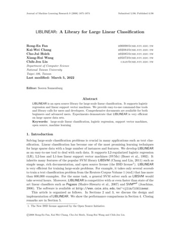
LIBLINEAR: A Library for Large Linear ClassificationAcknowledgmentsThis work was supported in part by the National Science Council of Taiwan via the grantNSC 95-2221-E-002-205-MY3.Appendix: Implementation Details and Practical GuideAppendix A. FormulationsThis section briefly describes classifiers supported in LIBLINEAR. Given training vectorsxi Rn , i 1, . . . , l in two class, and a vector y Rl such that yi {1, 1}, a linearclassifier generates a weight vector w as the model. The decision function is sgn wT x .A.1 Some Notes on the Bias TermBefore presenting all formulations, we briefly discuss the issue of the bias term in the model.Traditionally in classifiers such as SVM, the discriminant function of the classifier includesa bias term, b. For high-dimensional data it is known that with/without a bias term givesimilar performances. Therefore, the default setting of LIBLINEAR does not considera bias term in the model.For users stressing on having a bias term in the model, LIBLINEAR handles this termby augmenting the vector w and each instance xi with an additional dimension: wT [wT , b], xTi [xTi , B], where B is a constant specified by the user. The optimizationproblem becomes Xl1 T1 2xwminw w b C; i , yi ).(2)ξ(i 1bBw,b22After version 2.40, for some optimization methods, users can choose not to regularize thebias term. Then the optimization problem is Xl1 Txwminw w Cξ(; i , yi ).(3)i 1bBw,b2In the following subsections, we only consider the formulation in which the bias term isnot included.A.2 L2-regularized L1- and L2-loss Support Vector ClassificationL2-regularized L1-loss SVC solves the following primal problem:lminwX1 Tw w C(max(0, 1 yi wT xi )),2i 1whereas L2-regularized L2-loss SVC solves the following primal problem:lminwX1 Tw w C(max(0, 1 yi wT xi ))2 .2i 1A.1(4)

Fan, Chang, Hsieh, Wang and LinTheir dual forms are:minαsubject to1 Tα Q̄α eT α20 αi U, i 1, . . . , l.where e is the vector of all ones, Q̄ Q D, D is a diagonal matrix, and Qij yi yj xTi xj .For L1-loss SVC, U C and Dii 0, i. For L2-loss SVC, U and Dii 1/(2C), i.A.3 L2-regularized Logistic RegressionL2-regularized LR solves the following unconstrained optimization problem:lminwX1 TTw w Clog(1 e yi w xi ).2(5)i 1Its dual form is:minαsubject tolXXX1 Tα Qα αi log αi (C αi ) log(C αi ) C log C2i:αi 0i 1i:αi C(6)0 αi C, i 1, . . . , l.A.4 L1-regularized L2-loss Support Vector ClassificationL1 regularization generates a sparse solution w. L1-regularized L2-loss SVC solves thefollowing primal problem:minwkwk1 ClX(max(0, 1 yi wT xi ))2 .(7)i 1where k · k1 denotes the 1-norm.A.5 L1-regularized Logistic RegressionL1-regularized LR solves the following unconstrained optimization problem:minwkwk1 ClXlog(1 e yi wTxi).(8)i 1where k · k1 denotes the 1-norm.A.6 L2-regularized L1- and L2-loss Support Vector RegressionSupport vector regression (SVR) considers a problem similar to (1), but yi is a real valueinstead of 1 or 1. L2-regularized SVR solves the following primal problems:( PC li 1 (max(0, yi wT xi )) if using L1 loss,1 Tw w minPw2C li 1 (max(0, yi wT xi ))2 if using L2 loss,A.2

LIBLINEAR: A Library for Large Linear Classificationwhere 0 is a parameter to specify the sensitiveness of the loss.Their dual forms are:minα ,α subject to Q̄ Q α 1 αα y T (α α ) eT (α α ) Q Q̄α 20 αi , αi (9) U, i 1, . . . , l,where e is the vector of all ones, Q̄ Q D, Q Rl l is a matrix with Qij xTi xj , D isa diagonal matrix, Dii 012C(C, and U if using L1-loss SVR,if using L2-loss SVR.Rather than (9), in LIBLINEAR, we consider the following problem.minβsubject to1 Tβ Q̄β y T β kβk12 U βi U, i 1, . . . , l,(10)where β Rl and k · k1 denotes the 1-norm. It can be shown that an optimal solution of(10) leads to the following optimal solution of (9).αi max(βi , 0)andαi max( βi , 0).Appendix B. L2-regularized L1- and L2-loss SVM (Solving Dual)See Hsieh et al. (2008) for details of a dual coordinate descent method.Appendix C. L2-regularized Logistic Regression (Solving Primal)From versions 1.0 to 2.30, a trust region Newton method was considered. Some details areas follows. The main algorithm was developed in Lin et al. (2008). After version 2.11, the trust-region update rule is improved by the setting proposedin Hsia et al. (2017). After version 2.20, the convergence of conjugate gradient method is improved byapplying a preconditioning technique proposed in Hsia et al. (2018).After version 2.40, the trust-region Newton method is replaced by a line-search Newtonmethod. Details are in Galli and Lin (2021) and the release notes of LIBLINEAR 2.40 (Galliand Lin, 2020).A.3

Fan, Chang, Hsieh, Wang and LinAppendix D. L2-regularized L2-loss SVM (Solving Primal)The algorithm is the same as the Newton methods for logistic regression (trust-region Newton in Lin et al. (2008) before version 2.30 and line-search Newton in Galli and Lin (2021)after version 2.40). The only difference is the formulas of gradient and Hessian-vectorproducts. We list them here.The objective function is in (4). Its gradient isTw 2CXI,:(XI,: w yI ),(11) T x1 . TTwhere I {i 1 yi w xi 0} is an index set, y [y1 , . . . , yl ] , and X . .xTlEq. (4) is differentiable but not twice differentiable. To apply the Newton method, weconsider the following generalized Hessian of (4):TI 2CX T DX I 2CXI,:DI,I XI,: ,(12)where I is the identity matrix and D is a diagonal matrix with the following diagonalelements:(1 if i I,Dii 0 if i / I.The Hessian-vector product between the generalized Hessian and a vector s is:Ts 2CXI,:(DI,I (XI,: s)) .(13)Appendix E. Multi-class SVM by Crammer and SingerKeerthi et al. (2008) extend the coordinate descent method to a sequential dual methodfor a multi-class SVM formulation by Crammer and Singer. However, our implementationis slightly different from the one in Keerthi et al. (2008). In the following sections, wedescribe the formulation and the implementation details, including the stopping condition(Appendix E.4) and the shrinking strategy (Appendix E.5).E.1 FormulationsGiven a set of instance-label pairs (xi , yi ), i 1, . . . , l, xi Rn , yi {1, . . . , k}, Crammerand Singer (2000) proposed a multi-class approach by solving the following optimizationproblem:minwm ,ξisubject toklX1X Twm wm Cξi2m 1Twyi xi whereemiTwmxi(0 1 i 1mei ξi ,if yi m,if yi 6 m.A.4i 1, . . . , l,(14)

LIBLINEAR: A Library for Large Linear ClassificationThe decision function isTarg max wmx.m 1,.,kThe dual of (14) is:kl XkX1Xmkwm k2 emi αi2minαsubject tom 1i 1 m 1kXαim 0, i 1, . . . , lm 1αim Cymi , i 1, . . . , l, m(15) 1, . . . , k,wherewm lXαim xi , m,α [α11 , . . . , α1k , . . . , αl1 , . . . , αlk ]T .(16)i 1andCymi(0 Cif yi 6 m,if yi m.(17)Keerthi et al. (2008) proposed a sequential dual method to efficiently solve (15). Ourimplementation is based on this paper. The main differences are the sub-problem solverand the shrinking strategy.E.2 The Sequential Dual Method for (15)The optimization problem (15) has kl variables, which are very large. Therefore, we extendthe coordinate descent method to decomposes α into blocks [ᾱ1 , . . . , ᾱl ], whereᾱi [αi1 , . . . , αik ]T , i 1, . . . , l.Each time we select an index i and aim at minimizing the following sub-problem formed byᾱi :minᾱisubject tokX1A(αim )2 Bm αim2m 1kXαim 0,m 1αim Cymi , m {1, . . . , k},whereTmA xTi xi and Bm wmxi emi Aαi .In (18), A and Bm are constants obtained using α of the previous iteration.A.5(18)

Fan, Chang, Hsieh, Wang and LinAlgorithm 1 The coordinate descent method for (15) Given α and the corresponding wm While α is not optimal, (outer iteration)1. Randomly permute {1, . . . , l} to {π(1), . . . , π(l)}2. For i π(1), . . . , π(l), (inner iteration)If ᾱi is active and xTi xi 6 0 (i.e., A 6 0)– Solve a Ui -variable sub-problem (19)– Maintain wm for all m by (20)Since bounded variables (i.e., αim Cymi , m / Ui ) can be shrunken during training, weUiminimize with respect to a sub-vector ᾱi , where Ui {1, . . . , k} is an index set. That is,we solve the following Ui -variable sub-problem while fixing other variables:minUᾱi isubject toX 1A(αim )2 Bm αim2m UiXXαim ,αim m Uiαim (19)m U/ iCymi , m Ui .Notice that there are two situations that we do not solve the sub-problem of index i. First,if Ui 2, then the whole ᾱi is fixed by the equality constraint in (19). So we can shrinkthe whole vector ᾱi while training. Second, if A 0, then xi 0 and (16) shows thatthe value of αim does not affect wm for all m. So the value of ᾱi is independent of othervariables and does not affect the final model. Thus we do not need to solve ᾱi for thosexi 0.Similar to Hsieh et al. (2008), we consider a random permutation heuristic. Thatis, instead of solving sub-problems in the order of ᾱ1 , . . . ᾱl , we permute {1, . . . l} to{π(1), . . . π(l)}, and solve sub-problems in the order of ᾱπ(1) , . . . , ᾱπ(l) . Past results showthat such a heuristic gives faster convergence.We discuss our sub-problem solver in Appendix E.3. After solving the sub-problem, ifmα̂i is the old value and αim is the value after updating, we maintain wm , defined in (16),bywm wm (αim α̂im )yi xi .(20)To save the computational time, we collect elements satisfying αim 6 α̂im before doing (20).The procedure is described in Algorithm 1.E.3 Solving the sub-problem (19)We adopt the algorithm in Crammer and Singer (2000) but use a rather simple way as inLee and Lin (2013) to illustrate it. The KKT conditions of (19) indicate that there areA.6

LIBLINEAR: A Library for Large Linear ClassificationAlgorithm 2 Solving the sub-problem Given A, B Compute D by (27) Sort D in decreasing order; assume D has elements D1 , D2 , . . . , D Ui r 2, β D1 AC While r Ui and β/(r 1) Dr1. β β Dr2. r r 1 β β/(r 1) αim min(Cymi , (β Bm )/A), mscalars β, ρm , m Ui such thatXαim m Uiρm (Cymi Aαim Bmαimαim ) XCymi ,m U/ imCyi , m(21) Ui ,(22) 0, ρm 0, m Ui ,(23) β ρm , m Ui .(24)Using (22), equations (23) and (24) are equivalent toAαim Bm β 0, if αim Cymi , m Ui ,Aαim Bm β ACymi Bm β 0, ifαim(25) Cymi , m Ui .(26)Now KKT conditions become (21)-(22), and (25)-(26). For simplicity, we defineDm Bm ACymi , m 1, . . . , k.(27)If β is known, then we can show thatαim min(Cymi ,β Bm)A(28)satisfies all KKT conditions except (21). Clearly, the way to get αim in (28) gives αim Cymi , m Ui , so (22) holds. From (28), whenβ Bm Cymi , which is equivalent to β Dm ,Awe haveαim β Bm Cymi , which implies β Bm Aαim .AA.7(29)

Fan, Chang, Hsieh, Wang and LinThus, (25) is satisfied. Otherwise, β Dm and αim Cymi satisfies (26).The remaining task is how to find β such that (21) holds. From (21) and (25) we obtainXXX(β Bm ) (ACymi ACymi ).m:m Uimαmi Cyim:m Uiα Cymim:m U/ iThen,XXβ m:m Uimαmi CyiDm XACymim 1m:m Uimαmi Cyi kXDm AC.m:m Uimαmi CyiHence,Pβ mm Ui ,αmi CyiDm AC {m m Ui , αim Cymi } .(30)Combining (30) and (26), we begin with a set Φ φ, and then sequentially add oneindex m to Φ by the decreasing order of Dm , m 1, . . . , k, m 6 yi untilXDm ACh m Φ max Dm . Φ m Φ/(31)Let β h when (31) is satisfied. Algorithm 2 lists the details for solving the sub-problem(19). To prove (21), it is sufficient to show that β and αim , m Ui obtained by Algorithm2 satisfy (30). This is equivalent to showing that the final Φ satisfiesΦ {m m Ui , αim Cymi }.From (28) and (29), we prove the following equivalent result.β Dm , m Φ and β Dm , m / Φ.(32)The second inequality immediately follows from (31). For the first, assume t is the lastelement added to Φ. When it is considered, (31) is not satisfied yet, soXDm ACm Φ\{t} Φ 1 Dt .(33)Using (33) and the fact that elements in Φ are added in the decreasing order of Dm ,XXDm AC Dm Dt ACm Φm Φ\{t} ( Φ 1)Dt Dt Φ Dt Φ Ds , s Φ.Thus, we have the first inequality in (32).With all KKT conditions satisfied, Algorithm 2 obtains an optimal solution of (19).A.8

LIBLINEAR: A Library for Large Linear ClassificationE.4 Stopping ConditionThe KKT optimality conditions of (15) imply that there are b1 , . . . , bl R such that for alli 1, . . . , l, m 1, . . . , k,Tmmwmxi emi bi 0 if αi Ci ,Tmmwmxi emi bi 0 if αi Ci .LetGmi f (α)T wmxi emi , i, m, αimthe optimality of α holds if and only ifmax Gmi mminmm:αmi CiGmi 0, i.(34)At each inner iteration, we first compute Gmi and define:minG minmm:αmi CimGmi , maxG max Gi , Si maxG minG.mThen the stopping condition for a tolerance 0 can be checked bymax Si .i(35)Note that maxG and minG are calculated based on the latest α (i.e., α after each inneriteration).E.5 Shrinking StrategyThe shrinking technique reduces the size of the problem without considering some boundedvariables. Eq. (34) suggests that we can shrink αim out if αim satisfies the following condition:αim Cymi and Gmi minG.(36)Then we solve a Ui -variable sub-problem (19). To implement this strategy, we maintain anl k index array alpha index and an l array activesize i, such that activesize i[i] Ui . We let the first activesize i[i] elements in alpha index[i] are active indices, andothers are shrunken indices. Moreover, we need to maintain an l-variable array y index,such thatalphaindex[i][y index[i]] yi .(37)When we shrink a index alpha index[i][m] out, we first find the largest m̄ such that m̄ activesize i[i] and alpha index[i][m̄] does not satisfy the shrinking condition (36), thenswap the two elements and decrease activesize i[i] by 1. Note that if we swap index yi , weneed to maintain y index[i] to ensure (37). For the instance level shrinking and randompermutation, we also maintain a index array index and a variable activesize similar toalpha index and activesize i, respectively. We let the first activesize elements ofindex be active indices, while others be shrunken indices. When Ui , the active size of ᾱi ,A.9

Fan, Chang, Hsieh, Wang and LinAlgorithm 3 Shrinking strategy Given Begin with shrink max(1, 10 ), start from all T rue While1. For all active ᾱi(a) Do shrinking and calculate Si(b) stopping max(stopping, Si )(c) Optimize over active variables in ᾱi2. If stopping shrink(a)(b)(c)(d)If stopping and start from all is T rue, BREAKTake all shrunken variables backstart from all T rue shrink max( , shrink /2)Else(a) start from all F alseis less than 2 (activesize i[i] 2), we swap this index with the last active element inindex, and decrease activesize by 1.However, experiments show that (36) is too aggressive. There are too many wronglyshrunken variables. To deal with this problem, we use an -cooling strategy. Given apre-specified stopping tolerance , we begin with shrink max(1, 10 )and decrease it by a factor of 2 in each graded step until shrink .The program ends if the stopping condition (35) is satisfied. But we can exactly compute(35) only when there are no shrunken variables. Thus the process stops under the followingtwo conditions:1. None of the instances is shrunken in the beginning of the loop.2. (35) is satisfied.Our shrinking strategy is in Algorithm 3.Regarding the random permutation, we permute the first activesize elements of indexat each outer iteration, and then sequentially solve the sub-problems.Appendix F. L1-regularized L2-loss Support Vector MachinesIn this section, we describe details of a coordinate descent method for L1-regularized L2-losssupport vector machines. The problem formulation is in (7). Our procedure is similar toA.10

LIBLINEAR: A Library for Large Linear ClassificationChang et al. (2008) for L2-regularized L2-loss SVM, but we make certain modifications tohandle the non-differentiability due to the L1 regularization. It is also related to Tseng andYun (2009). See detailed discussions of theoretical properties in Yuan et al. (2010).Definebi (w) 1 yi wT xi and I(w) {i bi (w) 0}.The one-variable sub-problem for the jth variable is a function of z:f (w zej ) f (w)X wj z wj CXbi (w zej )2 Cbi (w)2i I(w)i I(w zej ) wj z Lj (z; w) constant1 wj z L0j (0; w)z L00j (0; w)z 2 constant,2(38)whereej [0, . . . , 0, 1, 0, . . . , 0]T Rn , {z }(39)j 1XLj (z; w) Cbi (w zej )2 ,i I(w zej )L0j (0; w) 2CXyi xij bi (w),i I(w)andL00j (0; w) max(2CXx2ij , 10 12 ).(40)i I(w)PNote that Lj (z; w) is differentiable but not twice differentiable, so 2C i I(w) x2ij in (40)is a generalized second derivative (Chang et al., 2008) at z 0. This value may be zeroif xij 0, i I(w), so we further make it strictly positive. The Newton direction fromminimizing (38) is 0L (0;w) 1 jif L0j (0; w) 1 L00j (0; w)wj , L0 00j (0;w)d Lj (0;w) 1if L0j (0; w) 1 L00j (0; w)wj ,L00 j (0;w) wotherwise.jSee the derivation in (Yuan et al., 2010, Appendix B). We then conduct a line searchprocedure to check if d, βd, β 2 d, . . . , satisfy the following sufficient decrease condition:XX wj β t d wj Cbi (w β t dej )2 Cbi (w)2i I(w β t dej )i I(w)(41) t0 σβ Lj (0; w)d wj d wj ,A.11

Fan, Chang, Hsieh, Wang and Linwhere t 0, 1, 2, . . . , β (0, 1), and σ (0, 1). From Chang et al. (2008, Lemma 5),XC2bi (w dej ) ClXbi (w) C(x2ij )d2 L0j (0; w)d.2i I(w)i I(w dej )We can precomputeXPl2i 1 xiji 1and checklX wj β t d wj C(x2ij )(β t d)2 L0j (0; w)β t di 1 σβ t(42) L0j (0; w)d wj d wj ,before (41). Note that checking (42) is very cheap. The main cost in checking (41) is oncalculating bi (w β t dej ), i. To save the number of operations, if bi (w) is available, onecan usebi (w β t dej ) bi (w) (β t d)yi xij .(43)Therefore, we store and maintain bi (w) in an array. Since bi (w) is used in every linesearch step, we cannot override its contents. After the line search procedure, we mustrun (43) again to update bi (w). That is, the same operation (43) is run twice, where thefirst is for checking the sufficient decrease condition and the second is for updating bi (w).Alternatively, one can use another array to store bi (w β t dej ) and copy its contents to thearray for bi (w) in the end of the line search procedure. We propose the following trick touse only one array and avoid the duplicated computation of (43). Frombi (w dej ) bi (w) dyi xij ,bi (w βdej ) bi (w dej ) (d βd)yi xij ,bi (w β 2 dej ) bi (w βdej ) (βd β 2 d)yi xij ,.(44)at each line search step, we obtain bi (w β t dej ) from bi (w β t 1 dej ) in order to check thesufficient decrease condition (41). If the condition is satisfied, then the bi array already hasvalues needed for the next sub-problem. If the condition is not satisfied, using bi (w β t dej )on the right-hand side of the equality (44), we can obtain bi (w β t 1 dej ) for the next linesearch step. Therefore, we can simultaneously check the sufficient decrease condition andupdate the bi array. A summary of the pro

Journal of Machine Learning Research 9 (2008) 1871-1874 Submitted 5/08; Published 8/08 LIBLINEAR: A Library for Large Linear Classi cation Rong-En Fan b90098@csie.ntu.edu.tw Kai-Wei Chang b92084@csie.ntu.edu.tw Cho-Jui Hsieh b92085@csie.ntu.edu.tw Xiang-Rui Wang r95073@csie.ntu.edu.tw Chih-Jen Lin cjlin@csie.ntu.edu.tw Department of Computer Science