Transcription
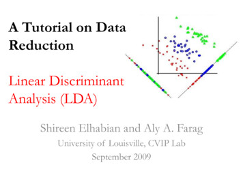
A Tutorial on DataReductionLinear DiscriminantAnalysis (LDA)Shireen Elhabian and Aly A. FaragUniversity of Louisville, CVIP LabSeptember 2009
Outline LDA objective Recall PCA Now LDA LDA Two Classes– Counter example LDA C Classes– Illustrative Example LDA vs PCA Example Limitations of LDA
LDA Objective The objective of LDAdimensionality reduction istoperform– So what, PCA does this L However, we want to preserve as much of theclass discriminatory information as possible.– OK, that’s new, let dwell deeper J
In PCA, the main idea to re-express the available dataset toextract the relevant information by reducing the redundancyand minimize the noise. We didn’t care about whether this dataset represent features from oneor more classes, i.e. the discrimination power was not taken intoconsideration while we were talking about PCA. In PCA, we had a dataset matrix X with dimensions mxn, wherecolumns represent different data samples. We first started by subtracting the mean to have a zero mean dataset,then we computed the covariance matrix Sx XXT. Eigen values and eigen vectors were then computed for Sx. Hence thenew basis vectors are those eigen vectors with highest eigen values,where the number of those vectors was our choice. Thus, using the new basis, we can project the dataset onto a lessdimensional space with more powerful data representation.m - dimensional data vectorRecall PCAn – feature vectors(data samples)
Now LDA Consider a pattern classification problem, where we have Cclasses, e.g. seabass, tuna, salmon Each class has Ni m-dimensional samples, where i 1,2, , C. Hence we have a set of m-dimensional samples {x1, x2, , xNi}belong to class ωi. Stacking these samples from different classes into one big fatmatrix X such that each column represents one sample. We seek to obtain a transformation of X to Y throughprojecting the samples in X onto a hyperplane withdimension C-1. Let’s see what does this mean?
LDA Two ClassesThe two classes are not wellseparated when projected ontothis line Assume we have m-dimensional samples {x1,x2, , xN}, N1 of which belong to ω1 andN2 belong to ω2. We seek to obtain a scalar y by projectingthe samples x onto a line (C-1 space, C 2).y wT xThis line succeeded in separatingthe two classes and in the meantime reducing thedimensionality of our problemfrom two features (x1,x2) to only ascalar value y.é x1 ùê. úwhere x ê úê. úê úë xm ûandé w1 ùê . úw ê úê . úê úë wm û– where w is the projection vectors used to project xto y.Of all the possible lines we would like toselect the one that maximizes theseparability of the scalars.
LDA Two Classes In order to find a good projection vector, we need to define ameasure of separation between the projections. The mean vector of each class in x and y feature space is:µ i1NiåxxÎwiandµ i1Niåy yÎwi1Ni wTåw wTxÎ1Nixiåw x w µTxÎii– i.e. projecting x to y will lead to projecting the mean of x to the mean ofy. We could then choose the distance between the projected meansas our objective functionJ (w) µ 1 - µ 2 wT µ1 - wT µ2 wT µ1 - µ2()
LDA Two Classes However, the distance between the projected means is not a verygood measure since it does not take into account the standarddeviation within the classes.This axis yields better class separabilityThis axis has a larger distance between means
LDA Two Classes The solution proposed by Fisher is to maximize a function thatrepresents the difference between the means, normalized by ameasure of the within-class variability, or the so-called scatter. For each class we define the scatter, an equivalent of thevariance, as; (sum of square differences between the projected samples and their classmean). si 2 )2(yµåiyÎwi s 2 measures the variability within class ω after projecting it oniithe y-space.s1 s2 measures the variability within the two Thus classes at hand after projection, hence it is called within-class scatterof the projected samples.22
LDA Two Classes The Fisher linear discriminant is defined asthe linear function wTx that maximizes thecriterion function: (the distance between theprojected means normalized by the withinclass scatter of the projected samples.2 µ 1 - µ2J ( w) 2 2s s1 2Therefore, we will be looking for a projectionwhere examples from the same class areprojected very close to each other and, at thesame time, the projected means are as fartherapart as possible
LDA Two Classes In order to find the optimum projection w*, we need to expressJ(w) as an explicit function of w. We will define a measure of the scatter in multivariate featurespace x which are denoted as scatter matrices;Si å (x - µi )(x - µi )T2 µ 1 - µ2J ( w) 2 2s s12xÎwiS w S1 S 2 Where Si is the covariance matrix of class ωi, and Sw is called thewithin-class scatter matrix.
LDA Two Classes Now, the scatter of the projection y can then be expressed as a function ofthe scatter matrix in feature space x.2 µ 1 - µ22J ( w) 2 222TT s ss y-µ w x-w µiåw (yÎii)åw (xÎi)1i å w (x - µi )(x - µi ) wTTxÎwiæT ö w çç å ( x - µi )(x - µi ) w wT Si wè xÎwiøT 22TTTT s1 s2 w S1w w S 2 w w (S1 S 2 )w w SW w SWWhere S W is the within-class scatter matrix of the projected samples y.2
LDA Two Classes Similarly, the difference between the projected means (in y-space) can beexpressed in terms of the means in the original feature space (x-space).(µ 1 - µ 2) (w µ2T1- w µ2T)2 wT (µ1 - µ 2 )(µ1 - µ 2 ) w !!!#!!!"2 µ 1 - µ2J ( w) 2 2s s12TSB w SB w SBT The matrix SB is called the between-class scatter of the original samples/featurevectors, while S B is the between-class scatter of the projected samples y. Since SB is the outer product of two vectors, its rank is at most one.
LDA Two Classes We can finally express the Fisher criterion in terms of SW and SBas:2 µ 1 - µ2wT S B wJ ( w) 2 2 Ts1 s2w SW w Hence J(w) is a measure of the difference between classmeans (encoded in the between-class scatter matrix)normalized by a measure of the within-class scatter matrix.
LDA Two Classes To find the maximum of J(w), we differentiate and equate tozero. dd æ wT S B w öçç T 0J ( w) dwdw è w SW w ø(() () ()()) ()ddTTÞ w SW ww SB w - w SB wwT SW w 0dwdwÞ wT SW w 2 S B w - wT S B w 2 SW w 0TDividing by 2 wT SW w :æ wT SW w öæ wT S B w ö S B w - çç T SW w 0Þ çç Tè w SW w øè w SW w øÞ S B w - J ( w) SW w 0Þ SW-1S B w - J ( w) w 0
LDA Two Classes Solving the generalized eigen value problemSW-1S B w lwwhere l J ( w) scalaryieldsTæwSB w ö* SW-1 (µ1 - µ2 )w arg max J ( w) arg maxçç Twwè w SW w ø This is known as Fisher’s Linear Discriminant, although it is not adiscriminant but rather a specific choice of direction for the projectionof the data down to one dimension. Using the same notation as PCA, the solution will be the eigen-1vector(s) of S X SW S B
LDA Two Classes - Example Compute the Linear Discriminant projection for the following twodimensional dataset.– Samples for class ω1 : X1 (x1,x2) {(4,2),(2,4),(2,3),(3,6),(4,4)}– Sample for class ω2 : X2 (x1,x2) 345x1678910
LDA Two Classes - Example The classes mean are :1µ1 N11 éæ 4 ö æ 2 ö æ 2 ö æ 3 ö æ 4 öù æ 3 öx êçç çç çç çç çç ú çç å5 ëè 2 ø è 4 ø è 3 ø è 6 ø è 4 øû è 3.8 øxÎw11µ2 N21 éæ 9 ö æ 6 ö æ 9 ö æ 8 ö æ10 öù æ 8.4 öx êçç çç çç çç çç ú çç å5 ëè10 ø è 8 ø è 5 ø è 7 ø è 8 øû è 7.6 øxÎw 2
LDA Two Classes - Example Covariance matrix of the first class:S1 åw (x - µ )(x - µ )TxÎ1112éæ 4 ö æ 3 öù éæ 2 ö æ 3 öù êçç - çç ú êçç - çç úëè 2 ø è 3.8 øû ëè 4 ø è 3.8 øû222éæ 2 ö æ 3 öù éæ 3 ö æ 3 öù éæ 4 ö æ 3 öù êçç - çç ú êçç - çç ú êçç - çç úëè 3 ø è 3.8 øû ëè 6 ø è 3.8 øû ëè 4 ø è 3.8 øû- 0.25 öæ 1 çç2.2 øè - 0.252
LDA Two Classes - Example Covariance matrix of the second class:S2 åw (x - µ )(x - µ )TxÎ2222éæ 9 ö æ 8.4 öù éæ 6 ö æ 8.4 öù êçç - çç ú êçç - çç úëè10 ø è 7.6 øû ëè 8 ø è 7.6 øû222éæ 9 ö æ 8.4 öù éæ 8 ö æ 8.4 öù éæ10 ö æ 8.4 öù êçç - çç ú êçç - çç ú êçç - çç úëè 5 ø è 7.6 øû ëè 7 ø è 7.6 øû ëè 8 ø è 7.6 øû- 0.05 öæ 2.3 çç3.3 øè - 0.052
LDA Two Classes - Example Within-class scatter matrix:- 0.25 ö æ 2.3- 0.05 öæ 1 çç S w S1 S 2 çç2.2 ø è - 0.053.3 øè - 0.25æ 3.3 - 0.3 ö ççè - 0.3 5.5 ø
LDA Two Classes - Example Between-class scatter matrix:S B (µ1 - µ 2 )(µ1 - µ 2 )Téæ 3 ö æ 8.4 öù éæ 3 ö æ 8.4 öù êçç - çç ú êçç - çç úëè 3.8 ø è 7.6 øû ëè 3.8 ø è 7.6 øûæ - 5.4 ö (- 5.4 - 3.8) ççè - 3.8 øæ 29.16 20.52 ö ççè 20.52 14.44 øT
LDA Two Classes - Example The LDA projection is then obtained as the solution of the generalized eigenvalue problem-1SW S B w lwÞ SW-1S B - lI 0æ 3 .3 - 0 .3 ö Þ ççè - 0.3 5.5 ø-1æ 29.16 20.52 ö æ 1 0 öçç - l çç 0è 20.52 14.44 ø è 0 1 øæ 0.3045 0.0166 öæ 29.16 20.52 ö æ 1 0 ö çç - l çç 0Þ ççè 0.0166 0.1827 øè 20.52 14.44 ø è 0 1 ø6.489 öæ 9.2213 - l Þ çç2.9794 - l øè 4.2339 (9.2213 - l )(2.9794 - l ) - 6.489 4.2339 0Þ l2 - 12.2007l 0 Þ l (l - 12.2007 ) 0Þ l1 0, l2 12.2007
LDA Two Classes - Example Henceæ w1 öæ 9.2213 6.489 öçç w1 0! çç l1 è w2 øè 4.2339 2.9794 øandæ w1 öæ 9.2213 6.489 öçç çç w2 12. 2007%""#è 4.2339 2.9794 øè w2 øl2Thus;æ - 0.5755 ö w1 ççè 0.8178 ø andæ 0.9088 ö w*w2 ççè 0.4173 øThe optimal projection is the one that given maximum λ J(w)
LDA Two Classes - ExampleOr directly;-1æ 3.3 - 0.3 ö éæ 3 ö æ 8.4 öù êçç - çç úw S (µ1 - µ 2 ) ççè - 0.3 5.5 ø ëè 3.8 ø è 7.6 øûæ 0.3045 0.0166 öæ - 5.4 ö çç ççè 0.0166 0.1827 øè - 3.8 ø*-1Wæ 0.9088 ö ççè 0.4173 ø
LDA - ProjectionClasses PDF : using the LDA projection vector with the other eigen value 8.8818e-0160.35The projection vectorcorresponding to thesmallest eigen value0.30.25LDA projection vector with the other eigen value 8.8818e-01610p(y wi )0.290.15870.16x20.05540-43-2-101y234Using this vector leads tobad separabilitybetween the two classes210-7-3-6-5-4-3-2-1012x134567891056
LDA - Projection0.4The projection vectorcorresponding to thehighest eigen valueClasses PDF : using the LDA projection vector with highest eigen value 12.20070.350.30.25LDA projection vector with the highest eigen value 12.2007p(y wi )1090.15870.126x0.20.05504510y3Using this vector leads togood separabilitybetween the two classes21000123456x17891015
LDA C-Classes Now, we have C-classes instead of just two. We are now seeking (C-1) projections [y1, y2, , yC-1] by meansof (C-1) projection vectors wi. wi can be arranged by columns into a projection matrix W [w1 w2 wC-1] such that:yi w xTiÞy W xTé x1 ùé y1 ùê . úê . úúwhere xm 1 ê ú, yC -1 1 êê . úê . úê úêúxyë mûë C -1 ûand Wm C -1 [w1 w2 . wC -1 ]
LDA C-Classes If we have n-feature vectors, we can stack them into one matrixas follows;Y WT XwhereX m né x11ê.ê ê.ê 1êë xmx12.xm2. x1n ùú. . ú. . únú. xm úû, YC -1 nand Wm C -1 [w1 w2 . wC -1 ]é y11ê.ê ê .ê 1êë yC -1y12.yC2 -1y1n ùú. ú. ún ú. yC -1 úû.
LDA – C-Classes Recall the two classes case, thewithin-class scatter was computed as:S w S1 S2Example of two-dimensionalfeatures (m 2), with threeclasses C 3.µ1x2 This can be generalized in the Cclasses case as:µ3µ2CSW å Sii 1whereandSi T()()xµxµåiiSw2xÎwi1µi Niåw xxÎiNi : number of data samplesin class ωi.x1
LDA – C-Classes Recall the two classes case, the betweenclass scatter was computed as:S B (µ1 - µ 2 )(µ1 - µ 2 )T µ1x2For C-classes case, we will measure thebetween-class scatter with respect to themean of all classes as follows:Cµµ3µ2S B å N i (µi - µ )(µi - µ )Ti 111whereµ åx N "xN1andµi xåN i xÎwiExample of two-dimensionalfeatures (m 2), with threeclasses C 3.å N i µi"xSw2x1N: number of all data .Ni : number of data samplesin class ωi.
LDA – C-Classes Similarly,– We can define the mean vectors for the projected samples y as:µ i 1Niåyandµ yÎwi1yåN "y– While the scatter matrices for the projected samples y will be:C CTSW å Si å å ( y - µ i )( y - µ i )i 1i 1 yÎwiC TS B å N i (µ i - µ )(µ i - µ )i 1
LDA – C-Classes Recall in two-classes case, we have expressed the scatter matrices of theprojected samples in terms of those of the original samples as: SW W T SWW S B W T S BWThis still hold in C-classes case. Recall that we are looking for a projection that maximizes the ratio ofbetween-class to within-class scatter. Since the projection is no longer a scalar (it has C-1 dimensions), we then usethe determinant of the scatter matrices to obtain a scalar objective function: SBW T S BWJ (W ) TW SW WSW And we will seek the projection W* that maximizes this ratio.
LDA – C-Classes To find the maximum of J(W), we differentiate with respect to W and equateto zero. Recall in two-classes case, we solved the eigen value problem.SW-1S B w lw For C-classes case, we have C-1 projection vectors, hence the eigen valueproblem can be generalized to the C-classes case as:SW-1S B wi li wi where l J ( w) scalarwhere li J ( wi ) scalarandi 1,2,.C - 1Thus, It can be shown that the optimal projection matrix W* is the one whosecolumns are the eigenvectors corresponding to the largest eigen values of thefollowing generalized eigen value problem:SW-1S BW * lW *where l J (W * ) scalarand[W * w1* w2* . wC* -1]
Illustration – 3 Classes Let’s generate a dataset for eachclass to simulate the three classesshownµ1x2 For each class do the following,– Use the random number generatorto generate a uniform stream of500 samples that follows U(0,1).µµ3µ2– Using the Box-Muller approach,x1convert the generated uniformstream to N(0,1).– Then use the method of eigen valuesand eigen vectors to manipulate thestandard normal to have the requiredmean vector and covariance matrix .– Estimate the mean and covariancematrix of the resulted dataset.
Dataset Generation By visual inspection of the figure,classes parameters (means andcovariance matrices can be given asfollows:Overall meané5ùµ ê úë5ûµ1x2µµ2é- 3ùé- 2.5ùé7 ùµ1 µ ê ú , µ 2 µ êú , µ 3 µ ê5 ú73.5ë ûëûë ûæ 5 - 1ö S1 ççNegative covariance to lead to data samples distributed along the y -x line.33èøæ 4 0öZero covariance to lead to data samples distributed horizontally. S 2 ççè 0 4øæ 3.5 1 ö S3 ççè 3 2.5 øµ3Positive covariance to lead to data samples distributed along the y x line.x1
In Matlab J
It’s Working Jµ1x220µµ215X2 - the second featureµ310x150-5-50510X1 - the first feature1520
Computing LDA Projection VectorsRecall CSW å Sii 1whereSi µi andT()()xµxµåiixÎwi1Niåw xxÎiCS B å N i (µi - µ )(µi - µ )-1WS SBTi 111whereµ åx N "xN1andµi åxN i xÎwiåN µ"xii
Let’s visualize the projection vectors W25X2 - the second feature20151050-5-10-15-10-50510X1 - the first feature152025
Projection y WTxAlong first projection vector0.4Classes PDF : using the first projection vector with eigen value 4508.20890.350.3p(y wi )0.250.20.150.10.050-50510y152025
Projection y WTxAlong second projection vectorClasses PDF : using the second projection vector with eigen value 1878.85110.40.350.3p(y wi )0.250.20.150.10.050-10-505y101520
Which is Better?!!! Apparently, the projection vector that has the highest eigenvalue provides higher discrimination power between classesClasses PDF : using the first projection vector with eigen value 4508.2089Classes PDF : using the second projection vector with eigen value 1878.85110.40.350.350.30.30.250.25p(y wi )p(y wi -505y101520
PCA vs LDA
Limitations of LDA L LDA produces at most C-1 feature projections– If the classification error estimates establish that more features are needed, some other method must beemployed to provide those additional featuresLDA is a parametric method since it assumes unimodal Gaussian likelihoods–If the distributions are significantly non-Gaussian, the LDA projections will not be able to preserve anycomplex structure of the data, which may be needed for classification.
Limitations of LDA L LDA will fail when the discriminatory information is not in the mean butrather in the variance of the data
Thank You
LDA Objective The objective of LDA is to perform dimensionalityreduction -Sowhat,PCAdoesthisL However,wewanttopreserveasmuchofthe .
