Transcription
Chapter EighteenDiscriminant and Logit AnalysisCopyright 2010 Pearson Education, Inc. publishing as Prentice Hall18-1
Direct marketing scenario Every year, the DM company sends to one annualcatalog, four seasonal catalogs, and a number ofcalalogs for holiday seasons. The company has a list of 10 million potentialbuyers. The response rate is on average 5%. Who should receive a catalog? (mostly likely tobuy) How are buyers different from nonbuyers? Who are most likely to default?.Copyright 2010 Pearson Education, Inc. publishing as Prentice Hall18-2
Similarities and Differences between ANOVA,Regression, and Discriminant AnalysisTable 18.1SimilaritiesNumber ofdependentvariablesNumber ofindependentvariablesANOVAREGRESSION eDifferencesNature of thedependentMetricMetricvariablesNature of theindependent Categorical MetricvariablesCopyright 2010 Pearson Education, Inc. publishing as Prentice HallCategoricalMetric (or binary, dummies)18-3
Discriminant AnalysisDiscriminant analysis is a technique for analyzing data whenthe criterion or dependent variable is categorical and thepredictor or independent variables are interval in nature.The objectives of discriminant analysis are as follows: Development of discriminant functions, or linearcombinations of the predictor or independent variables, whichwill best discriminate between the categories of the criterion ordependent variable (groups). (buyers vs. nonbuyers) Examination of whether significant differences exist among thegroups, in terms of the predictor variables. Determination of which predictor variables contribute to mostof the intergroup differences. Classification of cases to one of the groups based on the valuesof the predictor variables. Evaluation of the accuracy of classification.Copyright 2010 Pearson Education, Inc. publishing as Prentice Hall18-4
Discriminant Analysis When the criterion variable has two categories, the techniqueis known as two-group discriminant analysis.When three or more categories are involved, the technique isreferred to as multiple discriminant analysis.The main distinction is that, in the two-group case, it ispossible to derive only one discriminant function. In multiplediscriminant analysis, more than one function may becomputed. In general, with G groups and k predictors, it ispossible to estimate up to the smaller of G - 1, or k,discriminant functions.The first function has the highest ratio of between-groups towithin-groups sum of squares. The second function,uncorrelated with the first, has the second highest ratio, andso on. However, not all the functions may be statisticallysignificant.Copyright 2010 Pearson Education, Inc. publishing as Prentice Hall18-5
Geometric InterpretationFig. 18.1G1X21 11 11 1 111211112 22212222 222222G2G1G2X1DCopyright 2010 Pearson Education, Inc. publishing as Prentice Hall18-6
Discriminant Analysis ModelThe discriminant analysis model involves linear combinations ofthe following form:D b0 b1X1 b2X2 b3X3 . . . bkXkWhere:D discriminant scoreb 's discriminant coefficient or weightX 's predictor or independent variable The coefficients, or weights (b), are estimated so that the groupsdiffer as much as possible on the values of the discriminant function. This occurs when the ratio of between-group sum of squares towithin-group sum of squares for the discriminant scores is at amaximum.Copyright 2010 Pearson Education, Inc. publishing as Prentice Hall18-7
Statistics Associated withDiscriminant Analysis Canonical correlation. Canonical correlation measuresthe extent of association between the discriminant scoresand the groups. It is a measure of association between thesingle discriminant function and the set of dummy variablesthat define the group membership. Centroid. The centroid is the mean values for thediscriminant scores for a particular group. There are asmany centroids as there are groups, as there is one for eachgroup. The means for a group on all the functions are thegroup centroids. Classification matrix. Sometimes also called confusion orprediction matrix, the classification matrix contains thenumber of correctly classified and misclassified cases.Copyright 2010 Pearson Education, Inc. publishing as Prentice Hall18-8
Statistics Associated with DiscriminantAnalysis Discriminant function coefficients. The discriminantfunction coefficients (unstandardized) are the multipliers ofvariables, when the variables are in the original units ofmeasurement. Discriminant scores. The unstandardized coefficients aremultiplied by the values of the variables. These productsare summed and added to the constant term to obtain thediscriminant scores. Eigenvalue. For each discriminant function, the Eigenvalueis the ratio of between-group to within-group sums ofsquares. Large Eigenvalues imply superior functions.Copyright 2010 Pearson Education, Inc. publishing as Prentice Hall18-9
Statistics Associated with Discriminant Analysis F values and their significance. These are calculated froma one-way ANOVA, with the grouping variable serving as thecategorical independent variable. Each predictor, in turn,serves as the metric dependent variable in the ANOVA. Group means and group standard deviations. These arecomputed for each predictor for each group. Pooled within-group correlation matrix. The pooledwithin-group correlation matrix is computed by averagingthe separate covariance matrices for all the groups.Copyright 2010 Pearson Education, Inc. publishing as Prentice Hall18-10
Statistics Associated with Discriminant Analysis Standardized discriminant function coefficients. Thestandardized discriminant function coefficients are the discriminantfunction coefficients and are used as the multipliers when the variableshave been standardized to a mean of 0 and a variance of 1. Structure correlations. Also referred to as discriminant loadings,the structure correlations represent the simple correlations betweenthe predictors and the discriminant function. Total correlation matrix. If the cases are treated as if they werefrom a single sample and the correlations computed, a total correlationmatrix is obtained. Wilks'λ . Sometimes also called the U statistic, Wilks' λ for eachpredictor is the ratio of the within-group sum of squares to the totalsum of squares. Its value varies between 0 and 1. Large valuesof λ (near 1) indicate that group means do not seem to be different.Small values of λ (near 0) indicate that the group means seem to bedifferent.Copyright 2010 Pearson Education, Inc. publishing as Prentice Hall18-11
Conducting Discriminant AnalysisFig. 18.2Formulate the ProblemEstimate the Discriminant Function CoefficientsDetermine the Significance of the Discriminant FunctionInterpret the ResultsAssess Validity of Discriminant AnalysisCopyright 2010 Pearson Education, Inc. publishing as Prentice Hall18-12
Conducting Discriminant AnalysisFormulate the Problem Identify the objectives, the criterion variable, and theindependent variables.The criterion variable must consist of two or more mutuallyexclusive and collectively exhaustive categories.The predictor variables should be selected based on atheoretical model or previous research, or the experience ofthe researcher.One part of the sample, called the estimation or analysissample, is used for estimation of the discriminant function.The other part, called the holdout or validation sample, isreserved for validating the discriminant function.Often the distribution of the number of cases in the analysisand validation samples follows the distribution in the totalsample.Copyright 2010 Pearson Education, Inc. publishing as Prentice Hall18-13
Information on Resort Visits: AnalysisSampleTable 1111AnnualFamilyIncome( mportance Household Age ofAttachedSizeHead ofto FamilyHouseholdVacation875567345678826Copyright 2010 Pearson Education, Inc. publishing as Prentice mountSpent onFamilyVacationM (2)H (3)H (3)L (1)H (3)H (3)M (2)M (2)H (3)H (3)H (3)H (3)M (2)H (3)H (3)18-14
Table 18.2, cont.Information on Resort Visits: Analysis 222222222222222AnnualFamilyIncome( mportance Household Age ofAttachedSizeHead ofto FamilyHouseholdVacation435266254713823Copyright 2010 Pearson Education, Inc. publishing as Prentice mountSpent onFamilyVacationL (1)L (1)M (2)M (2)M (2)L (1)M (2)L (1)L (1)L (1)M (2)M (2)L (1)L (1)L (1)18-15
Information on Resort Visits:Holdout SampleTable lFamilyIncome( .2AttitudeTowardTravel476565456272Importance Household Age ofAttachedSizeHead ofto FamilyHouseholdVacation747466335632Copyright 2010 Pearson Education, Inc. publishing as Prentice t onFamilyVacationM(2)H (3)M(2)M(2)H (3)H (3)L (1)L (1)H (3)L (1)M(2)L (1)18-16
Conducting Discriminant AnalysisEstimate the Discriminant Function Coefficients The direct method involves estimating thediscriminant function so that all thepredictors are included simultaneously. In stepwise discriminant analysis, thepredictor variables are entered sequentially,based on their ability to discriminate amonggroups.Copyright 2010 Pearson Education, Inc. publishing as Prentice Hall18-17
Results of Two-Group Discriminant AnalysisINCOMETRAVEL 04.333334.866674.333332.800003.56667Table 18.4GROUP 1.93333Group Standard 1801.978041.820522.051712.09981Pooled Within-Groups Correlation EAGE1.000000.197450.091480.08887- 770628.271018.57395AGE1.00000Wilks' (U-statistic) and univariate F ratio with 1 and 28 degrees of 2572Copyright 2010 Pearson Education, Inc. publishing as Prentice HallCont.18-18
Results of Two-Group Discriminant AnalysisTable 18.4, cont.CANONICAL DISCRIMINANT FUNCTIONSFunction1*Eigenvalue1.7862% ofVariance100.00Cum Canonical AfterWilks'%Correlation Functionλ: 00 .3589100.000.8007:Chi-square df Significance26.13050.0001* marks the 1 canonical discriminant functions remaining in the analysis.Standard Canonical Discriminant Function 010.096110.233290.469110.20922Structure Matrix:Pooled within-groups correlations between discriminating variables & canonical discriminant functions(variables ordered by size of correlation within .540960.346070.213370.16354Copyright 2010 Pearson Education, Inc. publishing as Prentice HallCont.18-19
Results of Two-Group Discriminant AnalysisTable 18.4, cont.Unstandardized Canonical Discriminant Function CoefficientsFUNC 75476Canonical discriminant functions evaluated at group means (group centroids)GroupFUNC 111.291182-1.29118Classification results for cases selected for use in analysisPredictedActual GroupNo. of 500.0%15100.0%Percent of grouped cases correctly classified: 90.00%Cont.Copyright 2010 Pearson Education, Inc. publishing as Prentice Hall18-20
Results of Two-Group Discriminant AnalysisTable 18.4, cont.Classification Results for cases not selected for use inthe analysis (holdout sample)PredictedActual Group No. of .0%6100.0%Percent of grouped cases correctly classified: 83.33%.Copyright 2010 Pearson Education, Inc. publishing as Prentice Hall18-21
Conducting Discriminant AnalysisInterpret the Results The interpretation of the discriminant weights, or coefficients, is similarto that in multiple regression analysis.Given the multicollinearity in the predictor variables, there is nounambiguous measure of the relative importance of the predictors indiscriminating between the groups.With this caveat in mind, we can obtain some idea of the relativeimportance of the variables by examining the absolute magnitude of thestandardized discriminant function coefficients.Some idea of the relative importance of the predictors can also beobtained by examining the structure correlations, also called canonicalloadings or discriminant loadings. These simple correlations betweeneach predictor and the discriminant function represent the variance thatthe predictor shares with the function.Another aid to interpreting discriminant analysis results is to develop aCharacteristic profile for each group by describing each group interms of the group means for the predictor variables.Copyright 2010 Pearson Education, Inc. publishing as Prentice Hall18-22
Conducting Discriminant AnalysisAssess Validity of Discriminant Analysis Many computer programs, such as SPSS, offer a leave-oneout cross-validation option. The discriminant weights, estimated by using the analysissample, are multiplied by the values of the predictorvariables in the holdout sample to generate discriminantscores for the cases in the holdout sample. The cases arethen assigned to groups based on their discriminant scoresand an appropriate decision rule. The hit ratio, or thepercentage of cases correctly classified, can then bedetermined by summing the diagonal elements and dividingby the total number of cases. It is helpful to compare the percentage of cases correctlyclassified by discriminant analysis to the percentage thatwould be obtained by chance. Classification accuracyachieved by discriminant analysis should be at least 25%greater than that obtained by chance.Copyright 2010 Pearson Education, Inc. publishing as Prentice Hall18-23
Results of Three-Group Discriminant AnalysisTable 18.5Group 000Total51.216674.866674.933333.5666751.93333Group Standard 898.57395HSIZEAGEPooled Within-Groups Correlation .02512Copyright 2010 Pearson Education, Inc. publishing as Prentice Hall1.00000 Cont.18-24
All-Groups ScattergramFig. 18.3Across: Function 1Down: Function 24.0111 *1110.0112312 *2 212 223 *3 33333-4.0* indicates a groupcentroid-6.0-4.0 -2.00.0Copyright 2010 Pearson Education, Inc. publishing as Prentice Hall2.04.06.018-25
Territorial MapFig. 18.48.04.00.0-4.0-8.0-8.01313Across: Function 113Down: Function 21313* Indicates a13group centroid1311 3112 3112233* 1 1 1 2 2 2 2 3 3*112 *223233121 222331 122231 12 1 2 2233112222321122331112222331 121 2 222311223311122-6.0-4.0-2.00.0Copyright 2010 Pearson Education, Inc. publishing as Prentice Hall2.04.06.08.018-26
The Logit Model The dependent variable is binary andthere are several independent variablesthat are metric The binary logit model commonly dealswith the issue of how likely is anobservation to belong to each group(classification n prediction, buyer vsnonbuyer) It estimates the probability of anobservation belonging to a particulargroupCopyright 2010 Pearson Education, Inc. publishing as Prentice Hall18-27
Copyright 2010 Pearson Education, Inc. publishing as Prentice Hall18-28
Binary Logit Model FormulationThe probability of success may be modeled using the logit model as: P log a a 1 P e01X1 a2X2 . akXk P log a X 1 P nOreiii 0Copyright 2010 Pearson Education, Inc. publishing as Prentice Hall18-29
Model Formulationkexp( P 1 exp(i 0a Xii)k a Xi 0ii)Where:P Probability of successXi Independent variable iai parameter to be estimated.Copyright 2010 Pearson Education, Inc. publishing as Prentice Hall18-30
Properties of the Logit Model Although Xi may vary from to , P isconstrained to lie between 0 and 1. When Xi approaches , P approaches 0. When Xi approaches , P approaches 1. When OLS regression is used, P is notconstrained to lie between 0 and 1.Copyright 2010 Pearson Education, Inc. publishing as Prentice Hall18-31
Estimation and Model Fit The estimation procedure is called the maximum likelihoodmethod. Fit: Cox & Snell R Square and Nagelkerke R Square. Both these measures are similar to R2 in multipleregression. The Cox & Snell R Square can not equal 1.0, even if thefit is perfect. This limitation is overcome by the Nagelkerke R Square. Compare predicted and actual values of Y to determine thepercentage of correct predictions.Copyright 2010 Pearson Education, Inc. publishing as Prentice Hall18-32
Significance TestingThe significance of the estimated coefficients is based on Wald’s statistic.Wald (ai / SEai)2Where,ai logistical coefficient for that predictor variableSEai standard error of the logistical coefficientThe Wald statistic is chi-square distributed with 1 degree of freedom if thevariable is metric and the number of categories minus 1 if the variable isnonmetric.Copyright 2010 Pearson Education, Inc. publishing as Prentice Hall18-33
Interpretation of Coefficients If Xi is increased by one unit, the log oddswill change by ai units, when the effect ofother independent variables is heldconstant. The sign of ai will determine whether theprobability increases (if the sign is positive)or decreases (if the sign is negative) by thisamount.Copyright 2010 Pearson Education, Inc. publishing as Prentice Hall18-34
Explaining Brand LoyaltyTable 15165213464363553Copyright 2010 Pearson Education, Inc. publishing as Prentice HallShopping54454552442434532243453263223218-35
Results of Logistic RegressionTable 18.7Dependent Variable EncodingOriginal ValueNot LoyalInternal Value0Loyal1Model SummaryStep1-2 Loglikelihood23.471(a)Cox & SnellR Square.453Nagelkerke RSquare.604a Estimation terminated at iteration number 6 because parameter estimates changed by less than .001.Copyright 2010 Pearson Education, Inc. publishing as Prentice Hall18-36
Results of Logistic RegressionTable 18.7, cont.Classification Table aPredictedObservedStep 1 Loyalty to theBrandNot LoyalLoyalLoyalty to the BrandNot LoyalLoyal123312Overall PercentagePercentageCorrect80.080.080.0a. The cut value is .500Variables in the Equation ariable(s) entered on step 1: Brand, Product, Shopping.Copyright 2010 Pearson Education, Inc. publishing as Prentice Hall18-37
Table 18.5Results of Three-Group Discriminant AnalysisMultinomial Logistic regressionGroup 000Total51.216674.866674.933333.5666751.93333Group Standard 898.57395HSIZEAGEPooled Within-Groups Correlation 0.004740.22080CopyrightEducation, Inc. publishingHallAGE 2010 Pearson-0.20939-0.34022as Prentice-0.013261.00000-0.02512Cont.1.0000018-38
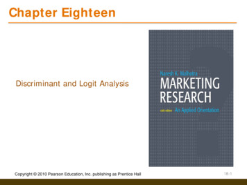
Chapter NineteenFactor AnalysisThe company asked 20 questionsabout casual dining and lifestyle.How are these questions relatedto one another? What are theimportant dimensions or factors?Copyright 2010 Pearson Education, Inc. publishing as Prentice Hall18-39
Factor Analysis Factor analysis is a general name denoting a class ofprocedures primarily used for data reduction and summarization. Factor analysis is an interdependence technique in that anentire set of interdependent relationships is examined withoutmaking the distinction between dependent and independentvariables. Factor analysis is used in the following circumstances: To identify underlying dimensions, or factors, that explainthe correlations among a set of variables. To identify a new, smaller, set of uncorrelated variables toreplace the original set of correlated variables in subsequentmultivariate analysis (regression or discriminant analysis). To identify a smaller set of salient variables from a larger setfor use in subsequent multivariate analysis.Copyright 2010 Pearson Education, Inc. publishing as Prentice Hall18-40
Factors Underlying Selected Psychographicsand LifestylesFig. 19.1Factor 2FootballBaseballEvening at homeFactor 1Go to a partyHome is best placePlaysCopyright 2010 Pearson Education, Inc. publishing as Prentice HallMovies18-41
Statistics Associated with Factor Analysis Bartlett's test of sphericity. Bartlett's test of sphericity is atest statistic used to examine the hypothesis that thevariables are uncorrelated in the population. In other words,the population correlation matrix is an identity matrix; eachvariable correlates perfectly with itself (r 1) but has nocorrelation with the other variables (r 0). Correlation matrix. A correlation matrix is a lower trianglematrix showing the simple correlations, r, between allpossible pairs of variables included in the analysis. Thediagonal elements, which are all 1, are usually omitted.Copyright 2010 Pearson Education, Inc. publishing as Prentice Hall18-42
Statistics Associated with Factor Analysis Communality. Communality is the amount of variance avariable shares with all the other variables being considered.This is also the proportion of variance explained by thecommon factors. Eigenvalue. The eigenvalue represents the total varianceexplained by each factor. Factor loadings. Factor loadings are simple correlationsbetween the variables and the factors. Factor loading plot. A factor loading plot is a plot of theoriginal variables using the factor loadings as coordinates. Factor matrix. A factor matrix contains the factor loadings ofall the variables on all the factors extracted.Copyright 2010 Pearson Education, Inc. publishing as Prentice Hall18-43
Statistics Associated with Factor Analysis Factor scores. Factor scores are composite scores estimatedfor each respondent on the derived factors. Kaiser-Meyer-Olkin (KMO) measure of samplingadequacy. The Kaiser-Meyer-Olkin (KMO) measure ofsampling adequacy is an index used to examine theappropriateness of factor analysis. High values (between 0.5and 1.0) indicate factor analysis is appropriate. Values below0.5 imply that factor analysis may not be appropriate. Percentage of variance. The percentage of the totalvariance attributed to each factor. Residuals are the differences between the observedcorrelations, as given in the input correlation matrix, and thereproduced correlations, as estimated from the factor matrix. Scree plot. A scree plot is a plot of the Eigenvalues againstthe number of factors in order of extraction.Copyright 2010 Pearson Education, Inc. publishing as Prentice Hall18-44
Conducting Factor AnalysisTable .007.006.003.00Copyright 2010 Pearson Education, Inc. publishing as Prentice 003.004.004.007.004.007.005.003.007.002.0018-45
Correlation MatrixTable 0Copyright 2010 Pearson Education, Inc. publishing as Prentice Hall18-46
Conducting Factor Analysis:Determine the Method of Factor Analysis In principal components analysis, the total variance in thedata is considered. The diagonal of the correlation matrixconsists of unities, and full variance is brought into the factormatrix. Principal components analysis is recommended whenthe primary concern is to determine the minimum number offactors that will account for maximum variance in the data foruse in subsequent multivariate analysis. The factors are calledprincipal components. In common factor analysis, the factors are estimated basedonly on the common variance. Communalities are inserted inthe diagonal of the correlation matrix. This method isappropriate when the primary concern is to identify theunderlying dimensions and the common variance is of interest.This method is also known as principal axis factoring.Copyright 2010 Pearson Education, Inc. publishing as Prentice Hall18-47
Results of Principal Components AnalysisTable 0.7390.8780.790Initial Eigen valuesFactor123456Eigen value2.7312.2180.4420.3410.1830.085Copyright 2010 Pearson Education, Inc. publishing as Prentice Hall% of variance45.52036.9697.3605.6883.0441.420Cumulat. %45.52082.48889.84895.53698.580100.00018-48
Results of Principal Components AnalysisTable 19.3, cont.Extraction Sums of Squared LoadingsFactor12Eigen value2.7312.218% of variance45.52036.969Cumulat. %45.52082.488Factor MatrixVariablesV1V2V3V4V5V6Factor 10.928-0.3010.936-0.342-0.869-0.177Factor 20.2530.7950.1310.789-0.3510.871Rotation Sums of Squared LoadingsFactor Eigenvalue % of variance12.68844.80222.26137.687Copyright 2010 Pearson Education, Inc. publishing as Prentice HallCumulat. %44.80282.48818-49
Results of Principal Components AnalysisTable 19.3, cont.Rotated Factor MatrixVariablesV1V2V3V4V5V6Factor 10.962-0.0570.934-0.098-0.9330.083Factor 2-0.0270.848-0.1460.845-0.0840.885Factor Score Coefficient MatrixVariablesV1V2V3V4V5V6Factor 10.358-0.0010.345-0.017-0.3500.052Copyright 2010 Pearson Education, Inc. publishing as Prentice HallFactor 20.0110.375-0.0430.377-0.0590.39518-50
Conducting Factor Analysis: Rotate Factors Although the initial or unrotated factor matrixindicates the relationship between the factors andindividual variables, it seldom results in factors thatcan be interpreted, because the factors arecorrelated with many variables. Therefore, throughrotation, the factor matrix is transformed into asimpler one that is easier to interpret. In rotating the factors, we would like each factor tohave nonzero, or significant, loadings orcoefficients for only some of the variables.Likewise, we would like each variable to havenonzero or significant loadings with only a fewfactors, if possible with only one. The rotation is called orthogonal rotation if theaxes are maintained at right angles.Copyright 2010 Pearson Education, Inc. publishing as Prentice Hall18-51
Conducting Factor Analysis: Rotate Factors The most commonly used method for rotation isthe varimax procedure. This is an orthogonalmethod of rotation that minimizes the number ofvariables with high loadings on a factor, therebyenhancing the interpretability of the factors.Orthogonal rotation results in factors that areuncorrelated. The rotation is called oblique rotation when theaxes are not maintained at right angles, and thefactors are correlated. Sometimes, allowing forcorrelations among factors can simplify the factorpattern matrix. Oblique rotation should be usedwhen factors in the population are likely to bestrongly correlated.Copyright 2010 Pearson Education, Inc. publishing as Prentice Hall18-52
Factor Matrix Before and After RotationFig. 19.5FactorsVariables1234561XXXXX2XXXX(a)High LoadingsBefore RotationCopyright 2010 Pearson Education, Inc. publishing as Prentice HallFactorsVariables1234561X2XXXXX(b)High LoadingsAfter Rotation18-53
Conducting Factor Analysis: Interpret Factors A factor can then be interpreted in terms ofthe variables that load high on it. Another useful aid in interpretation is to plotthe variables, using the factor loadings ascoordinates. Variables at the end of an axisare those that have high loadings on onlythat factor, and hence describe the factor.Copyright 2010 Pearson Education, Inc. publishing as Prentice Hall18-54
Chapter TwentyCluster AnalysisCopyright 2010 Pearson Education, Inc. publishing as Prentice Hall18-55
Copyright 2010 Pearson Education, Inc. publishing as Prentice Hall18-56
Chapter Outline1) Overview2) Basic Concept (e.g., segmentation without priorknown groups)3) Statistics Associated with Clust
Conducting Discriminant Analysis Estimate the Discriminant Function Coefficients The . direct method. involves estimating the discriminant function so that all the predictors are included simultaneously. In. stepwise discriminant analysis, the predictor variables are entered sequentially, based on their ability to discriminate among groups.