Transcription
Metodološki zvezki, Vol. 1, No. 1, 2004, 143-161Comparison of Logistic Regression and LinearDiscriminant Analysis: A Simulation StudyMaja Pohar1, Mateja Blas2, and Sandra Turk3AbstractTwo of the most widely used statistical methods for analyzingcategorical outcome variables are linear discriminant analysis and logisticregression. While both are appropriate for the development of linearclassification models, linear discriminant analysis makes more assumptionsabout the underlying data. Hence, it is assumed that logistic regression isthe more flexible and more robust method in case of violations of theseassumptions. In this paper we consider the problem of choosing between thetwo methods, and set some guidelines for proper choice. The comparisonbetween the methods is based on several measures of predictive accuracy.The performance of the methods is studied by simulations. We start with anexample where all the assumptions of the linear discriminant analysis aresatisfied and observe the impact of changes regarding the sample size,covariance matrix, Mahalanobis distance and direction of distance betweengroup means. Next, we compare the robustness of the methods towardscategorisation and non-normality of explanatory variables in a closelycontrolled way. We show that the results of LDA and LR are closewhenever the normality assumptions are not too badly violated, and setsome guidelines for recognizing these situations. We discuss theinappropriateness of LDA in all other cases.1IntroductionLinear discriminant analysis (LDA) and logistic regression (LR) are widely usedmultivariate statistical methods for analysis of data with categorical outcome1Department of Medical Informatics, University of Ljubljana; maja.pohar@mf.uni-lj.siPostgraduate student of Statistics, University of Ljubljana; mateja.blas@guest.arnes.si3Sandra Turk, Krka d.d., Novo mesto; sandra.turk@krka.biz2
144Maja Pohar, Mateja Blas, and Sandra Turkvariables. Both of them are appropriate for the development of linearclassification models, i.e. models associated with linear boundaries between thegroups.Nevertheless, the two methods differ in their basic idea. While LR makes noassumptions on the distribution of the explanatory data, LDA has been developedfor normally distributed explanatory variables. It is therefore reasonable to expectLDA to give better results in the case when the normality assumptions arefulfilled, but in all other situations LR should be more appropriate. The theoreticalproperties of LR and LDA are thoroughly dealt with in the literature, however thechoice of the method is often more related to the field of statistics than to theactual condition of fulfilled assumptions.The goal of this paper is not to discourage the current practice but rather to setsome guidelines as to when the choice of either one of the methods is stillappropriate. While LR is much more general and has a number of theoreticalproperties, LDA must be the better choice if we know the population is normallydistributed. However, in practice, the assumptions are nearly always violated, andwe have therefore tried to check the performance of both methods withsimulations. This kind of research demands a careful control, so we have decidedto study just a few chosen situations, trying to find a logic in the behaviour andthen to think about the expansion onto more general cases. We have confinedourselves to compare only the predictive power of the methods.The article is organized as follows. Section 2 briefly reviews LR and LDA andexplains their graphical representation. Section 3 details the criteria chosen tocompare both methods. Section 4 describes the process of the simulations. Theresults obtained are presented and discussed in Section 5, starting with the casewhere all the assumptions of LDA are fulfilled and continuing with cases wherenormality is violated in sense of categorization and skewness. It is shown howviolation of the assumptions of LDA affects both methods and how robust themethods are. The paper concludes with some guidelines for the choice between themodels and a discussion.2Logistic regression and linear discriminant analysisThe goal of LR is to find the best fitting and most parsimonious model to describethe relationship between the outcome (dependent or response variable) and a set ofindependent (predictor or explanatory) variables. The method is relatively robust,flexible and easily used, and it lends itself to a meaningful interpretation. In LR,unlike in the case of LDA, no assumptions are made regarding the distribution ofthe explanatory variables.Contrary to the popular beliefs, both methods can be applied to more than twocategories (Hosmer and Lemeshow, 1989, p. 216). To simplify, we only focus on
Comparison of Logistic Regression and Linear 145the case of a dichotomous outcome variable (Y). The LR model can be expressedasP(Yi 1 X i ) eβTXi1 eβ(2.1)TXiwhere the Yi are independent Bernoulli random variables. The coefficients of thismodel are estimated using the maximum likelihood method. LR is discussedfurther by Hosmer and Lemeshow (1989).Linear discriminant analysis can be used to determine which variablediscriminates between two or more classes, and to derive a classification model forpredicting the group membership of new observations (Worth and Cronin, 2003).For each of the groups, LDA assumes the explanatory variables to be normallydistributed with equal covariance matrices. The simplest LDA has two groups. Todiscriminate between them, a linear discriminant function that passes through thecentroids of the two groups can be used. LDA is discussed further by Kachigan(1991). The standard LDA model assumes that the conditional distribution of X yis multivariate normal with mean vector µy and common covariance matrix Σ.With some algebra we can show that we assign x to group 1 asP(1 x) where α and β coefficients are11 ( eα βx )(2.2) 1β (µ1 µ 0 )T 1π 1α log 1 (µ1 µ 0 )T 1 (µ1 µ 0 )π0 2(2.3)π1 and π0 are prior probabilities of belonging to group 1 and group 0. In practicethe parameters π1, π0, µ1, µ0 and Σ will be unknown, so we replace them by theirsample estimates, i. e.:n1n, πˆ 0 0 ,nn11µˆ 1 x1 x i , µˆ 0 x 0 n1 yi 1n0πˆ 1 ˆ (x y 1 iiy i 0(2.4),yi 0 x1 )( x i x1 ) ( x i x 0 )( x i x 0 )Ti xT /n (2.2) is equal in form to LR. Hence, the two methods do not differ in functionalform, they only differ in the estimation of coefficients.
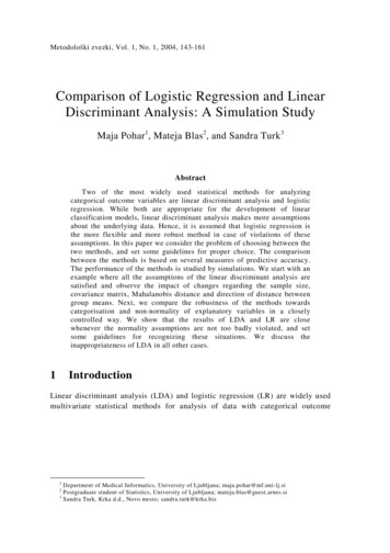
1462.1Maja Pohar, Mateja Blas, and Sandra TurkGraphical representation: An explanationWhen the values of α and β are known, the expression for a set of points withequal probability of allocation can be derived asT0.5 eα β x1 eα βT x 0 α β xT(2.5)-20x224In two-dimensional perspective this set of points is a line, while in threedimensions it is a plane.Figure 1 shows the scatterplot for two explanatory variables. Each of the twogroups is plotted with a different character. The linear borders presented arecalculated on the basis of the estimates of each method. The ellipses indicate thedistributions assumed by the LDA.logistic regressiondiscriminant analysis-2024x1Figure 1: The linear borders between the groups for LR (solid) and LDA (dotted line).3Comparison criteriaThe simplest and the most frequently used criterion for comparison between thetwo methods is classification error (percent of incorrectly classified objects; CE).However, classification error is a very insensitive and statistically inefficientmeasure (Harrell, 1997). The fact is that the classification error is usually nearlythe same in both methods, but, when differences exist, they are oftenoverestimated (for example, if the threshold for “yes” is 0.50, a prediction of 0.99rates the same as one of 0.51). The minimum information gained with theclassification error is in the case of categorical explanatory variables. Theboundary lines in figures below differ approximately equally in coefficients, butthe classification errors provide different information. In Figure 2a, one of the
Comparison of Logistic Regression and Linear 14754123x2312x245possible outcomes lies in the area where the lines are different, and therefore thepredictions will differ in all objects with this outcome. On the contrary, the areabetween the lines in Figure 2b covers none of the possible outcomes. Theclassification error therefore does not reveal any difference.1234512x1345x1Figure 2a and 2b: Examples of categorised explanatory variables.Since more information is needed regarding the predictive accuracy of themethods than just a binary classification rule, Harrell and Lee (1985) proposedfour different measures of comparing predictive accuracy of the two methods.These measures are indexes A, B, C and Q. They are better and more efficientcriteria for comparisons and they tell us how well the models discriminate betweenthe groups and/or how good the prediction is. Theoretical insight and experienceswith simulations revealed that some indexes are more and some less appropriate atdifferent assumptions. In this work, we focus on three measures of predictiveaccuracy, the B, C and Q indexes. Because of its intuitive clearness we sometimesadd the classification error (CE) as well.The C index is purely a measure of discrimination (discrimination refers to theability of a model to discriminate or separate values of Y). It is written as followsnn1C [I(Pj Pi ) I(Pj Pi )]/ n 0 n1i 1 j 12Y 0 Y 1i(3.1)jwhere Pk denotes an estimate of P(Yk 1 Xk) from (2.1) and I is an indicatorfunction.We can see that the value of the C index is independent of the actual groupmembership (Y), and as such it is only a measure of discrimination between thegroups, and not a measure of accuracy of prediction. A C index of 1 indicatesperfect discrimination; a C index of 0.5 indicates random prediction.
148Maja Pohar, Mateja Blas, and Sandra TurkThe B and Q indexes can be used to assess the accuracy of the outcomeprediction. The B index measures an average of squared difference between anestimated and actual value:B 1 (Pi Yi ) 2 / nn(3.2)i 1where Pi is a probability of classification into group i, Yi is the actual groupmembership (1 or 0), and n is the sample size of both populations. The values ofthe B index are on the interval [0,1], where 1 indicates perfect prediction. In thecase of random prediction in two equally sized groups, the value of the B index is0.75.The Q index is similar to the B index and is also a measure of predictiveaccuracy:Q 1 log 2 (Pi Y i (1 Pi )1 Yi ) / n .n(3.3)i 1A score of 1 of the Q index indicates perfect prediction. A Q index of 0 indicatesrandom predictions, and values less than 0 indicate worse than random predictions.When predicted probabilities of 0 or 1 exist, the Q index is undefined. The B, Cand Q indexes are discussed further by Harrell and Lee (1985).While the C index is purely a measure of discrimination, the B and Q indexes(besides discrimination) also consider accuracy of prediction. Hence, we canexpect these two indexes to be the most sensitive measures in our simulations.Instead of comparing the indexes directly, we will often focus only on theproportion of simulations in which LR predicts better than LDA. As we alwaysperform 50 simulations, this proportion will be statistically significant whenever itlies outside the interval [0.36, 0.64].44.1Description of the SimulationsBasic functionThe basic function enables us to draw random samples of size n and m from twomultivariate normal populations with different mean vectors, but equal covariancematrix Σ. The mean vector of one group is always set at (0,0). The distance to theother one is measured using Mahalanobis distance, while the direction is set as theangle (denoted by υ) to the direction of the eigenvector of the covariance matrix.Each sample is then randomly divided into two parts, a training and a testsample. The coefficents of LDA and LR are computed using the first sample andthen predictions are made in the second one. The sampling experiment isreplicated 50 times. Each time the indexes for both methods are computed. Finally,the average value of indexes and the proportion of simulations in which LRperforms better are recorded.
Comparison of Logistic Regression and Linear 4.2149CategorizationAfter sampling, the normally distributed variables can be categorised, either onlyone or both of them. The minimum and maximum value are computed, then thewhole interval is divided into a certain number of categories of equal size.4.3SkewnessAs in the case of categorization, we can also decide here to transform only one oftwo explanatory variables or both of them. The Box-Cox type of transformation(Box and Cox, 1964) is used to make normal distribution skewed.4.4RemarksTo ensure clarity of the graphical representation, we have confined ourselves to atwo- dimensional perspective, i.e. two explanatory variables. We have neverthelessmade some simulations in more dimensions, but the trends of the results seemed tofollow the same pattern.In most of the simulations we have also set an upper limit for the Mahalanobisdistance, in order to prevent LR from failing to converge and LDA from givingunreliable results.To simplify, we have fixed the two group sizes as the same. As unequally sizedgroups (or unequal a prori probabilities in LR) only shift the border line closer tothe smaller group (the one with the less probable outcome), this only impacts theconstant, while the coefficient estimates remain the same.All the simulations and computations were performed by using the statisticalsoftware package R.55.1ResultsComparison of methods when LDA assumptions are satisfiedWe start from the situation where both explanatory variables are normallydistributed. We observe the impact of changes connected with the parameters:sample size, covariance matrix, Mahalanobis distance and direction of distancebetween the group means.The sample size has the most obvious impact on the difference betweenmethods. LDA assumes normality and the errors it makes in prediction are onlydue to the errors in estimation of the mean and variance on the sample. On thecontrary, LR adapts itself to distribution and assumes nothing about it. Therefore,
150Maja Pohar, Mateja Blas, and Sandra Turkin the case of small samples, the difference between the distribution of the trainingsample and that of the test sample can be substantial. But, as the sample sizeincreases, the sampling distributions become more stable which leads to betterresults for the LR. Consequently, the results of the two methods are getting closerbecause the populations are normally distributed.Table 1: Simulation results for the effect of sample size 0LDA0.17000.16470.15270.15850.1543The proportion of simulations in which LR performs betterBCQCELR bettersameLR bettersameLR bettersameLR 01002001000 1 0 . 50. 5 ,1 υ π /42x200x2-2-3-2-1-1-10x2112133Parameters: Σ 0123x1Figure 3: The impact of sample size of n 50 (left), n 100 (middle) and n 200 (right).The results from Table 1 confirm the consideration above. As the sample sizeincreases, the LDA coefficient estimations become more accurate and therefore allfour indexes are improving (bold face is used to highlight the method thatperforms better). The LR indexes are increasing even faster, thus approachingthose of LDA. Decreasing difference between the two methods is best presentedwith the Q index, which is the most sensitive one. As the differences betweenindex means are negligible, it is also interesting to look at the proportion ofsimulations where LR performs better. It can be seen that the value of rates to
Comparison of Logistic Regression and Linear 151which we pay special attention, that of B index and of Q index, is constantlyincreasing.In the case of other changes (tables below) the results of the two methodsremain very close, in fact LDA is only a little bit better than LR. The exceptionappears in the case of large Mahalanobis distance presented in Table 4. We can seethat for low values of Mahalanobis distance LDA yields better results, but as thisdistance increases and it takes values above 2, LR performs better.Table 2: Simulation results for the effect of correlation between explanatoryvariables( σ he proportion of simulations in which LR performs betterBCQCELR bettersameLR bettersameLR bettersameLR 460.180.260.000.32same0.220.360.220.30Parameters: υ π /4, m n 50Table 3: Simulation results for the effect of direction of distance between groupmeans( υ ).Bν0Π /4Π /3Π /2ν0Π /4Π /3Π 5240.16440.1613LR0.16290.15790.15110.1579The proportion of simulations in which LR performs betterBCQCELR bettersameLR bettersameLR bettersameLR 360.300.240.000.32Parameters: Σ 1 0 . 50. 5 ,1 m n 50LDA0.16090.15650.14800.1569same0.360.180.340.30
152Maja Pohar, Mateja Blas, and Sandra TurkTable 4: Simulation results for the effect of Mahalanobis distance 16060.14860.12410.10260.0756The proportion of simulations in which LR performs betterBCQCELR bettersameLR bettersameLR bettersameLR 0.900.000.420.080.000.26Parameters: Σ 1 0 . 50. 5 ,1 00.380.300.240.40υ π /4, m n 50To sum up, we can say that in the case of normality LDA yields better resultsthan LR. However, for very large sample sizes the results of the two methodsbecome really close.5.2The effect of categorisationThe effect of categorisation is studied under the assumption that the explanatoryvariables are in fact normally distributed, but measured only discretely. Thismeans they only have a limited number of values or categories. When the numberof categories is big enough not to disturb the accuracy of the estimates, thecategorisation will not cause any changes in our results. But when the values areforced into just a few categories, we can expect more discrepancies.All the simulations in this section are performed in the following way: First,the values of the indexes for LR and LDA are calculated for the samples from thenormally distributed population. We start from the situation, where the LDAperforms better as shown in the previous section (in the tables, these results aredenoted with ). These samples are then categorised into a certain number ofcategories and the indexes are again calculated and compared.As expected, the effect of the categorisation depends somewhat on the datastructure (the correlation among the variables), but nevertheless, in all thesimulations similar trends can be observed.Linear discriminant analysis proves to be rather robust. Its prediction power isnot much lower when the values are in 5 or more categories, and it usually
Comparison of Logistic Regression and Linear 153-3-3-2-2-2-1-1-10x21x200x212123234performs better than LR. The story changes when the number of categories is low,and LR is the only appropriate choice in the binary case.The effect of categorisation also depends on the significance of the effect of acertain explanatory variable on the outcome. This is understandable – anonsignificant variable will not change the model if transformed. On the otherhand, if two covariates, equally powerful when predicting the result, arecategorised, each of them will have a similar impact on the result.-4-20x12-2-101x1234-3-2-101234x1Figure 4a, 4b and 4c: The basic situations used in the study. The ellipses describe thedistributions within the groups.We have studied the impact of categorisation in two extreme and oneintermediate case. Figures below present the situations that were the basis of oursimulations. Figure 4a presents two uncorrelated explanatory variables with asimilar impact on the outcome. In Figure 4b only one of the variables issignificant, while in Figure 4c the covariates are correlated and both have asignificant but different impact on the outcome variable.Table 5a summarizes the results of the situation shown in Figure 4c. The upperpart of this table contains the Q indexes for the case in which both covariates arecategorised. It can be seen that the categorisation into only two categoriesseverally lowers the predictive power of the two variables (the Q index falls closeto zero) and that this effect is greater with LDA. For better clarity, the lower partof this table concentrates only on the proportion of the simulations in which theLR performs better (with regard to index Q) and compares these results with thecategorisation of only one variable at a time. It is obvious that LR alwaysoutperforms LDA in the binary case. As discussed above, this effect is greaterwhen we categorise the more significant variable (x2) and even more so when wecategorise both explanatory variables.The results summed up in Table 5b are similar. The effect of both x 1 and x 2 issimilar and therefore the trends are even more comparable. However, logisticregression is not truly better even in the two category case. That is probably due tothe too big “head start” of LDA. When categorising both covariates the advantagesof LR are again more obvious.
154Maja Pohar, Mateja Blas, and Sandra TurkTable 5a: Simulation results for different number of categories (Figure 4c).QNum. of categ.LRLDALR .780.5850.12670.12810.46100.14670.15050.18 0.15530.15950.20The proportion of simulations in which LR performsbetter (Q index)Num. of .5850.300.260.46 0.200.200.20Parameters: Σ 1 0 . 50 . 5 , υ 0,1 m n 200Table 5b: Simulation results for different number of categories (Figure 4a).The proportion of simulations in which LR performsbetter (Q index)Num. of 0.260.24 0.260.260.260.460.32Parameters: Σ 1 0 , υ π /4, m n 200 01 Table 5c clearly shows the absence of any effect on the result when wecategorise an insignificant variable (x1). The results in the second and the thirdcolumn are practically the same, because categorising only x2 variable is the sameas categorising both.Table 5c: Simulation results for different number of categories (Figure 4b).The proportion of simulations in which LR performsbetter (Q index)Num. of .3450.200.300.30 0.260.200.20Parameters: Σ 1 0 , υ 0, m n 200 01
Comparison of Logistic Regression and Linear 155If the study of the categorisation effect is done by taking smaller samples, theadvantages of LDA are greater (see the previous section). Therefore they do nottail off even in the case of a small number of categories. Table 5d presents theresults of an identical situation as in the lower part of Table 5a, but the samplesize is shrunk to 100 units.Table 5d: Simulation results for different number of categories (Figure 4c).The proportion of simulations in which LR performsbetter (Q index)Num. of .2650.240.300.26 0.220.220.20Parameters: Σ 1 0 . 50 . 5 , υ 0,1 m n 100The results in this table tend to vary a bit. Too small a sample size, and at thesame time a small number of outcomes, causes the results to be unreliable. This iseven more obvious when the Mahalanobis distance is increased, because LR oftenhas problems with convergence.5.3The effect of non-normalityx24x262240020x264886101012In the case of categorical explanatory variables above, the assumption of normalityhas been preserved and only the consequences of discrete measurement have beenstudied. Now, we are interested in the robustness of LDA when the normalityassumptions are not met and in how much better can LR be in these cases. As nonnormality is a very broad term, we have confined ourselves to transforming normaldistributions with a Box-Cox transformation and thus making them skewed.Again we begin with the three situations shown in Figure 4 and transform theminto what is shown in Figure 5.05x1100510x102468x1Figure 5a, 5b and 5c: Examples of right skewed distributions (to make groups morediscernible, a part of the convex hull has been drawn for each of them).
156Maja Pohar, Mateja Blas, and Sandra TurkTable 6a: Simulation results for different degree of skewness (Figures 4c, 5c).QCS*LRLDALR .960.50.0505*Coefficient of skewnessParameters: Σ 1 0 . 50 . 5 , υ 0,1 m n 200The performance of LDA and LR does not depend on the sign of the skewness.Therefore we have used the same transformation function to check the impact ofthe extent of separation of the groups at the same time. Right skewness thus alsomean less separated groups. This is obvious in Table 6a, as index Q is constantlydecreasing.To be able to compare LR and LDA solely in terms of skewness we againfocus on the proportion of simulations where LR does better. Tables 6b, 6c and 6dshow the results for all the three cases we have described in Figures 4 and 5. Thefirst two columns always show the results when only one of the two explanatoryvariables is skewed, while in the third column both are transformed.The trends we can see are rather similar. When the skewness is small andtherefore the distribution close to normal, LDA performs better. But when theskewness increases, LR becomes more and more constantly better.Table 6b: Simulation results for different degree of skewness (Figures 4c, 5c).The proportion of simulations in which LR performsbetter (Q .380.420.600.40.520.540.880.580.5*Coefficient of skewness0.640.96Parameters: Σ 1 0 . 50 . 5 , υ 0,1 m n 200
Comparison of Logistic Regression and Linear 157If both explanatory variables are skewed, the highest value of skewness underwhich LDA is still more appropriate is about 0,2. We can observe that theseboundaries are the same regardless of the separation of the groups.If only one of the covariates is asymmetric and the other one is left as normal,the LDA is expectedly more robust – the interval widens a bit and the trends againremain similar with positive and negative skewness. The same effect on robustnesscan be seen by lowering the sample size as discussed in the previous sections.Table 6d again shows that transforming insignificant variables has no impacton the results. However, it is impossible to control the simulations to the extentwhere we could say anything exact about the boundaries depending on thesignificance of the variables.Table 6c: Simulation results for different degree of skewness (Figures 4a, 5a).The proportion of simulations in which LR performsbetter (Q .280.280.560.40.500.400.860.580.5*Coefficient of skewness0.500.94Parameters: Σ 1 0 , υ π /4, m n 200 01 Table 6d: Simulation results for different degree of skewness (Figures 4b, 5b).The proportion of simulations in which LR performsbetter (Q .260.620.600.40.260.920.920.50.26*Coefficient of skewness0.980.98Parameters: Σ 1 0 , υ 0, m n 200 01
Maja Pohar, Mateja Blas, and Sandra Turk05x21015158051015x1Figure 6: Right skewness with shifted centroids.In this study we have confined ourselves to situations where the use of eitherLDA or LR is sensible. Figure 6 presents a situation similar to the one in Figure4c, but with the centroids of the groups being shifted in a different direction.While we can imagine sensible linear boundaries on the Figures 5a, b and c, theboundary curve in Figure 6 is obviously not linear. Therefore more work should bedone before using LDA or LR.6Conclusions and discussionThe goal of this paper was to compare logistic regression and linear discriminantanalysis in order to set some guidelines to make the choice between the methodseasier.The methods do not differ in their functional forms. The difference rather liesin the estimation of the coefficients and we have focused our study on theirpredictive power.The literature offers several criteria for comparison of the two methods. Wehave discussed some of them and showed that the classification error, althoughmost frequently used, is not appropriate in our case. It is not sensitive enough andcan be biased. We preferred the B and Q indexes, both leading to similar res
Linear discriminant analysis (LDA) and logistic regression (LR) are widely used multivariate statistical methods for analysis of data with categorical outcome 1 Department of Medical Informatics, University of Ljubljana; maja.pohar@mf.uni-lj.si 2 Postgraduate student of Statistics, University of Ljubljana; mateja.blas@guest.arnes.si


![Advanced Analytics in Business [D0S07a] Big Data Platforms .](/img/28/3-20-20supervised-20learning.jpg)