Transcription
20STATISTICAL LEARNINGMETHODSIn which we view learning as a form of uncertain reasoning from observations.Part V pointed out the prevalence of uncertainty in real environments. Agents canhandle uncertainty by using the methods of probability and decision theory, but first theymust learn their probabilistic theories of the world from experience. This chapter explainshow they can do that. We will see how to formulate the learning task itself as a processof probabilistic inference (Section 20.1). We will see that a Bayesian view of learning isextremely powerful, providing general solutions to the problems of noise, overfitting, andoptimal prediction. It also takes into account the fact that a less-than-omniscient agent cannever be certain about which theory of the world is correct, yet must still make decisions byusing some theory of the world.We describe methods for learning probability models—primarily Bayesian networks—in Sections 20.2 and 20.3. Section 20.4 looks at learning methods that store and recall specificinstances. Section 20.5 covers neural network learning and Section 20.6 introduces kernelmachines. Some of the material in this chapter is fairly mathematical (requiring a basic understanding of multivariate calculus), although the general lessons can be understood withoutplunging into the details. It may benefit the reader at this point to review the material inChapters 13 and 14 and to peek at the mathematical background in Appendix A.20.1S TATISTICAL L EARNINGThe key concepts in this chapter, just as in Chapter 18, are data and hypotheses. Here, thedata are evidence—that is, instantiations of some or all of the random variables describingthe domain. The hypotheses are probabilistic theories of how the domain works, includinglogical theories as a special case.Let us consider a very simple example. Our favorite Surprise candy comes in twoflavors: cherry (yum) and lime (ugh). The candy manufacturer has a peculiar sense of humorand wraps each piece of candy in the same opaque wrapper, regardless of flavor. The candy issold in very large bags, of which there are known to be five kinds—again, indistinguishablefrom the outside:712
Section 20.1.Statistical Learningh1 :h2 :h3 :h4 :h5 :BAYESIAN LEARNING713100% cherry75% cherry 25% lime50% cherry 50% lime25% cherry 75% lime100% limeGiven a new bag of candy, the random variable H (for hypothesis) denotes the type of thebag, with possible values h1 through h5 . H is not directly observable, of course. As thepieces of candy are opened and inspected, data are revealed—D1 , D2 , . . ., DN , where eachDi is a random variable with possible values cherry and lime. The basic task faced by theagent is to predict the flavor of the next piece of candy.1 Despite its apparent triviality, thisscenario serves to introduce many of the major issues. The agent really does need to infer atheory of its world, albeit a very simple one.Bayesian learning simply calculates the probability of each hypothesis, given the data,and makes predictions on that basis. That is, the predictions are made by using all the hypotheses, weighted by their probabilities, rather than by using just a single “best” hypothesis.In this way, learning is reduced to probabilistic inference. Let D represent all the data, withobserved value d; then the probability of each hypothesis is obtained by Bayes’ rule:P (hi d) αP (d hi )P (hi ) .(20.1)Now, suppose we want to make a prediction about an unknown quantity X. Then we haveP(X d) XP(X d, hi )P(hi d) YP (dj hi ) .iHYPOTHESIS PRIORLIKELIHOODI.I.D.XiP(X hi )P (hi d) ,(20.2)where we have assumed that each hypothesis determines a probability distribution over X.This equation shows that predictions are weighted averages over the predictions of the individual hypotheses. The hypotheses themselves are essentially “intermediaries” between theraw data and the predictions. The key quantities in the Bayesian approach are the hypothesisprior, P (hi ), and the likelihood of the data under each hypothesis, P (d hi ).For our candy example, we will assume for the time being that the prior distributionover h1 , . . . , h5 is given by h0.1, 0.2, 0.4, 0.2, 0.1i, as advertised by the manufacturer. Thelikelihood of the data is calculated under the assumption that the observations are i.i.d.—thatis, independently and identically distributed—so thatP (d hi ) j(20.3)For example, suppose the bag is really an all-lime bag (h5 ) and the first 10 candies are alllime; then P (d h3 ) is 0.510 , because half the candies in an h3 bag are lime.2 Figure 20.1(a)shows how the posterior probabilities of the five hypotheses change as the sequence of 10lime candies is observed. Notice that the probabilities start out at their prior values, so h 3is initially the most likely choice and remains so after 1 lime candy is unwrapped. After 21Statistically sophisticated readers will recognize this scenario as a variant of the urn-and-ball setup. We findurns and balls less compelling than candy; furthermore, candy lends itself to other tasks, such as deciding whetherto trade the bag with a friend—see Exercise 20.3.2 We stated earlier that the bags of candy are very large; otherwise, the i.i.d. assumption fails to hold. Technically,it is more correct (but less hygienic) to rewrap each candy after inspection and return it to the bag.
10.80.6Probability that next candy is limeChapter 20.Posterior probability of hypothesis714P(h1 d)P(h2 d)P(h3 d)P(h4 d)P(h5 d)0.40.2002468Number of samples in d(a)10Statistical Learning Methods10.90.80.70.60.50.402468Number of samples in d10(b)Figure 20.1 (a) Posterior probabilities P (hi d1 , . . . , dN ) from Equation (20.1). The number of observations N ranges from 1 to 10, and each observation is of a lime candy. (b)Bayesian prediction P (dN 1 lime d1 , . . . , dN ) from Equation (20.2).MAXIMUM APOSTERIORIlime candies are unwrapped, h4 is most likely; after 3 or more, h5 (the dreaded all-lime bag)is the most likely. After 10 in a row, we are fairly certain of our fate. Figure 20.1(b) showsthe predicted probability that the next candy is lime, based on Equation (20.2). As we wouldexpect, it increases monotonically toward 1.The example shows that the true hypothesis eventually dominates the Bayesian prediction. This is characteristic of Bayesian learning. For any fixed prior that does not rule out thetrue hypothesis, the posterior probability of any false hypothesis will eventually vanish, simply because the probability of generating “uncharacteristic” data indefinitely is vanishinglysmall. (This point is analogous to one made in the discussion of PAC learning in Chapter 18.)More importantly, the Bayesian prediction is optimal, whether the data set be small or large.Given the hypothesis prior, any other prediction will be correct less often.The optimality of Bayesian learning comes at a price, of course. For real learningproblems, the hypothesis space is usually very large or infinite, as we saw in Chapter 18. Insome cases, the summation in Equation (20.2) (or integration, in the continuous case) can becarried out tractably, but in most cases we must resort to approximate or simplified methods.A very common approximation—one that is usually adopted in science—is to make predictions based on a single most probable hypothesis—that is, an hi that maximizes P (hi d).This is often called a maximum a posteriori or MAP (pronounced “em-ay-pee”) hypothesis. Predictions made according to an MAP hypothesis hMAP are approximately Bayesian tothe extent that P(X d) P(X hMAP ). In our candy example, hMAP h5 after three limecandies in a row, so the MAP learner then predicts that the fourth candy is lime with probability 1.0—a much more dangerous prediction than the Bayesian prediction of 0.8 shownin Figure 20.1. As more data arrive, the MAP and Bayesian predictions become closer, because the competitors to the MAP hypothesis become less and less probable. Although ourexample doesn’t show it, finding MAP hypotheses is often much easier than Bayesian learn-
Section 20.1.Statistical Learning715ing, because it requires solving an optimization problem instead of a large summation (orintegration) problem. We will see examples of this later in the chapter.In both Bayesian learning and MAP learning, the hypothesis prior P (hi ) plays an important role. We saw in Chapter 18 that overfitting can occur when the hypothesis spaceis too expressive, so that it contains many hypotheses that fit the data set well. Rather thanplacing an arbitrary limit on the hypotheses to be considered, Bayesian and MAP learningmethods use the prior to penalize complexity. Typically, more complex hypotheses have alower prior probability—in part because there are usually many more complex hypothesesthan simple hypotheses. On the other hand, more complex hypotheses have a greater capacity to fit the data. (In the extreme case, a lookup table can reproduce the data exactly withprobability 1.) Hence, the hypothesis prior embodies a trade-off between the complexity of ahypothesis and its degree of fit to the data.We can see the effect of this trade-off most clearly in the logical case, where H containsonly deterministic hypotheses. In that case, P (d hi ) is 1 if hi is consistent and 0 otherwise.Looking at Equation (20.1), we see that hMAP will then be the simplest logical theory thatis consistent with the data. Therefore, maximum a posteriori learning provides a naturalembodiment of Ockham’s razor.Another insight into the trade-off between complexity and degree of fit is obtainedby taking the logarithm of Equation (20.1). Choosing hMAP to maximize P (d hi )P (hi )is equivalent to minimizing log2 P (d hi ) log2 P (hi ) .MINIMUMDESCRIPTIONLENGTHMAXIMUMLIKELIHOODUsing the connection between information encoding and probability that we introduced inChapter 18, we see that the log2 P (hi ) term equals the number of bits required to specifythe hypothesis hi . Furthermore, log2 P (d hi ) is the additional number of bits requiredto specify the data, given the hypothesis. (To see this, consider that no bits are requiredif the hypothesis predicts the data exactly—as with h5 and the string of lime candies—andlog2 1 0.) Hence, MAP learning is choosing the hypothesis that provides maximum compression of the data. The same task is addressed more directly by the minimum descriptionlength, or MDL, learning method, which attempts to minimize the size of hypothesis anddata encodings rather than work with probabilities.A final simplification is provided by assuming a uniform prior over the space of hypotheses. In that case, MAP learning reduces to choosing an hi that maximizes P (d Hi ).This is called a maximum-likelihood (ML) hypothesis, hML . Maximum-likelihood learningis very common in statistics, a discipline in which many researchers distrust the subjectivenature of hypothesis priors. It is a reasonable approach when there is no reason to prefer onehypothesis over another a priori—for example, when all hypotheses are equally complex. Itprovides a good approximation to Bayesian and MAP learning when the data set is large,because the data swamps the prior distribution over hypotheses, but it has problems (as weshall see) with small data sets.
71620.2Chapter 20.Statistical Learning MethodsL EARNING WITH C OMPLETE DATAPARAMETERLEARNINGCOMPLETE DATAOur development of statistical learning methods begins with the simplest task: parameterlearning with complete data. A parameter learning task involves finding the numerical parameters for a probability model whose structure is fixed. For example, we might be interestedin learning the conditional probabilities in a Bayesian network with a given structure. Dataare complete when each data point contains values for every variable in the probability modelbeing learned. Complete data greatly simplify the problem of learning the parameters of acomplex model. We will also look briefly at the problem of learning structure.Maximum-likelihood parameter learning: Discrete modelsSuppose we buy a bag of lime and cherry candy from a new manufacturer whose lime–cherryproportions are completely unknown—that is, the fraction could be anywhere between 0 and1. In that case, we have a continuum of hypotheses. The parameter in this case, which wecall θ, is the proportion of cherry candies, and the hypothesis is hθ . (The proportion of limesis just 1 θ.) If we assume that all proportions are equally likely a priori, then a maximumlikelihood approach is reasonable. If we model the situation with a Bayesian network, weneed just one random variable, Flavor (the flavor of a randomly chosen candy from the bag).It has values cherry and lime, where the probability of cherry is θ (see Figure 20.2(a)). Nowsuppose we unwrap N candies, of which c are cherries and N c are limes. Accordingto Equation (20.3), the likelihood of this particular data set isP (d hθ ) NYj 1LOG LIKELIHOODP (dj hθ ) θc · (1 θ) .The maximum-likelihood hypothesis is given by the value of θ that maximizes this expression. The same value is obtained by maximizing the log likelihood,L(d hθ ) log P (d hθ ) NXj 1log P (dj hθ ) c log θ log(1 θ) .(By taking logarithms, we reduce the product to a sum over the data, which is usually easierto maximize.) To find the maximum-likelihood value of θ, we differentiate L with respect toθ and set the resulting expression to zero:c ccdL(d hθ ) 0 θ .dθθ 1 θc NIn English, then, the maximum-likelihood hypothesis hML asserts that the actual proportionof cherries in the bag is equal to the observed proportion in the candies unwrapped so far!It appears that we have done a lot of work to discover the obvious. In fact, though, wehave laid out one standard method for maximum-likelihood parameter learning:1. Write down an expression for the likelihood of the data as a function of the parameter(s).2. Write down the derivative of the log likelihood with respect to each parameter.3. Find the parameter values such that the derivatives are zero.
Section 20.2.Learning with Complete Data717P(F cherry)θP(F cherry)FlavorθFFlavorP(W red F)cherryθ1limeθ2Wrapper(a)(b)Figure 20.2 (a) Bayesian network model for the case of candies with an unknown proportion of cherries and limes. (b) Model for the case where the wrapper color depends (probabilistically) on the candy flavor.The trickiest step is usually the last. In our example, it was trivial, but we will see that inmany cases we need to resort to iterative solution algorithms or other numerical optimizationtechniques, as described in Chapter 4. The example also illustrates a significant problemwith maximum-likelihood learning in general: when the data set is small enough that someevents have not yet been observed—for instance, no cherry candies—the maximum likelihoodhypothesis assigns zero probability to those events. Various tricks are used to avoid thisproblem, such as initializing the counts for each event to 1 instead of zero.Let us look at another example. Suppose this new candy manufacturer wants to give alittle hint to the consumer and uses candy wrappers colored red and green. The Wrapper foreach candy is selected probabilistically, according to some unknown conditional distribution,depending on the flavor. The corresponding probability model is shown in Figure 20.2(b).Notice that it has three parameters: θ, θ1 , and θ2 . With these parameters, the likelihood ofseeing, say, a cherry candy in a green wrapper can be obtained from the standard semanticsfor Bayesian networks (page 495):P (Flavor cherry, Wrapper green hθ,θ1 ,θ2 ) P (Flavor cherry hθ,θ1 ,θ2 )P (Wrapper green Flavor cherry, hθ,θ1 ,θ2 ) θ · (1 θ1 ) .Now, we unwrap N candies, of which c are cherries and are limes. The wrapper counts areas follows: rc of the cherries have red wrappers and gc have green, while r of the limes havered and g have green. The likelihood of the data is given byP (d hθ,θ1 ,θ2 ) θc (1 θ) · θ1rc (1 θ1 )gc · θ2r (1 θ2 )g .This looks pretty horrible, but taking logarithms helps:L [c log θ log(1 θ)] [rc log θ1 gc log(1 θ1 )] [r log θ2 g log(1 θ2 )] .The benefit of taking logs is clear: the log likelihood is the sum of three terms, each of whichcontains a single parameter. When we take derivatives with respect to each parameter and set
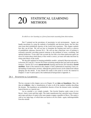
718Chapter 20.Statistical Learning Methodsthem to zero, we get three independent equations, each containing just one parameter: L θ L θ1 L θ2 c θ 1 θ 0gcrcθ1 1 θ1 g r θ2 1 θ2 00cθ c cθ1 rcr gc θ2 r r g. The solution for θ is the same as before. The solution for θ1 , the probability that a cherrycandy has a red wrapper, is the observed fraction of cherry candies with red wrappers, andsimilarly for θ2 .These results are very comforting, and it is easy to see that they can be extended to anyBayesian network whose conditional probabilities are represented as tables. The most important point is that, with complete data, the maximum-likelihood parameter learning problemfor a Bayesian network decomposes into separate learning problems, one for each parameter.3 The second point is that the parameter values for a variable, given its parents, are just theobserved frequencies of the variable values for each setting of the parent values. As before,we must be careful to avoid zeroes when the data set is small.Naive Bayes modelsProbably the most common Bayesian network model used in machine learning is the naiveBayes model. In this model, the “class” variable C (which is to be predicted) is the rootand the “attribute” variables Xi are the leaves. The model is “naive” because it assumes thatthe attributes are conditionally independent of each other, given the class. (The model inFigure 20.2(b) is a naive Bayes model with just one attribute.) Assuming Boolean variables,the parameters areθ P (C true), θi1 P (Xi true C true), θi2 P (Xi true C false).The maximum-likelihood parameter values are found in exactly the same way as for Figure 20.2(b). Once the model has been trained in this way, it can be used to classify new examples for which the class variable C is unobserved. With observed attribute values x 1 , . . . , xn ,the probability of each class is given byP(C x1 , . . . , xn ) α P(C)YiP(xi C) .A deterministic prediction can be obtained by choosing the most likely class. Figure 20.3shows the learning curve for this method when it is applied to the restaurant problem fromChapter 18. The method learns fairly well but not as well as decision-tree learning; this ispresumably because the true hypothesis—which is a decision tree—is not representable exactly using a naive Bayes model. Naive Bayes learning turns out to do surprisingly well in awide range of applications; the boosted version (Exercise 20.5) is one of the most effectivegeneral-purpose learning algorithms. Naive Bayes learning scales well to very large problems: with n Boolean attributes, there are just 2n 1 parameters, and no search is requiredto find hML , the maximum-likelihood naive Bayes hypothesis. Finally, naive Bayes learninghas no difficulty with noisy data and can give probabilistic predictions when appropriate.3See Exercise 20.7 for the nontabulated case, where each parameter affects several conditional probabilities.
Learning with Complete Data7191Proportion correct on test setSection 20.2.0.90.80.70.6Decision treeNaive Bayes0.50.40204060Training set size80100Figure 20.3 The learning curve for naive Bayes learning applied to the restaurant problemfrom Chapter 18; the learning curve for decision-tree learning is shown for comparison.Maximum-likelihood parameter learning: Continuous modelsContinuous probability models such as the linear-Gaussian model were introduced in Section 14.3. Because continuous variables are ubiquitous in real-world applications, it is important to know how to learn continuous models from data. The principles for maximumlikelihood learning are identical to those of the discrete case.Let us begin with a very simple case: learning the parameters of a Gaussian densityfunction on a single variable. That is, the data are generated as follows:(x µ)21e 2σ2 .P (x) 2πσThe parameters of this model are the mean µ and the standard deviation σ. (Notice that thenormalizing “constant” depends on σ, so we cannot ignore it.) Let the observed values bex1 , . . . , xN . Then the log likelihood isL N(xj µ)X (xj µ)21.log e 2σ2 N ( log 2π log σ) 2σ 22πσj 1j 1NX2Setting the derivatives to zero as usual, we obtain σ12PN L µ L σ Nσ j 1 (xj1σ3PN µ) 02j 1 (xj µ) 0 µ σ PjxjrNPj(xj µ)2N(20.4).That is, the maximum-likelihood value of the mean is the sample average and the maximumlikelihood value of the standard deviation is the square root of the sample variance. Again,these are comforting results that confirm “commonsense” practice.Now consider a linear Gaussian model with one continuous parent X and a continuouschild Y . As explained on page 502, Y has a Gaussian distribution whose mean dependslinearly on the value of X and whose standard deviation is fixed. To learn the conditional
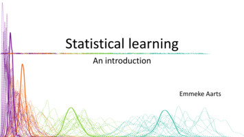
720Chapter 20.Statistical Learning Methods10.80.6yP(y x)43.532.521.510.500 0.20.40.4 0.60.8x1010.80.60.4 y0.20.2000.1 0.2 0.3 0.4 0.5 0.6 0.7 0.8 0.9x(a)1(b)Figure 20.4 (a) A linear Gaussian model described as y θ1 x θ2 plus Gaussian noisewith fixed variance. (b) A set of 50 data points generated from this model.distribution P (Y X), we can maximize the conditional likelihood(y (θ1 x θ2 ))212σ 2.(20.5)P (y x) e 2πσHere, the parameters are θ1 , θ2 , and σ. The data are a collection of (xj , yj ) pairs, as illustratedin Figure 20.4. Using the usual methods (Exercise 20.6), we can find the maximum-likelihoodvalues of the parameters. Here, we want to make a different point. If we consider just theparameters θ1 and θ2 that define the linear relationship between x and y, it becomes clear thatmaximizing the log likelihood with respect to these parameters is the same as minimizing thenumerator in the exponent of Equation (20.5):E NXj 1ERRORSUM OF SQUAREDERRORSLINEAR REGRESSION(yj (θ1 xj θ2 ))2 .The quantity (yj (θ1 xj θ2 )) is the error for (xj , yj )—that is, the difference between theactual value yj and the predicted value (θ1 xj θ2 )—so E is the well-known sum of squarederrors. This is the quantity that is minimized by the standard linear regression procedure.Now we can understand why: minimizing the sum of squared errors gives the maximumlikelihood straight-line model, provided that the data are generated with Gaussian noise offixed variance.Bayesian parameter learningMaximum-likelihood learning gives rise to some very simple procedures, but it has someserious deficiencies with small data sets. For example, after seeing one cherry candy, themaximum-likelihood hypothesis is that the bag is 100% cherry (i.e., θ 1.0). Unless one’shypothesis prior is that bags must be either all cherry or all lime, this is not a reasonableconclusion. The Bayesian approach to parameter learning places a hypothesis prior over thepossible values of the parameters and updates this distribution as data arrive.
Section 20.2.Learning with Complete Data2.57216[5,5]54[2,2]1.53[1,1]1[30,10]P(Θ θ)P(Θ θ)220.510000.20.40.6Parameter θ0.81[6,2][3,1]00.20.40.6Parameter θ(a)Figure 20.5BETA DISTRIBUTIONSHYPERPARAMETER1(b)Examples of the beta[a, b] distribution for different values of [a, b].The candy example in Figure 20.2(a) has one parameter, θ: the probability that a randomly selected piece of candy is cherry flavored. In the Bayesian view, θ is the (unknown)value of a random variable Θ; the hypothesis prior is just the prior distribution P(Θ). Thus,P (Θ θ) is the prior probability that the bag has a fraction θ of cherry candies.If the parameter θ can be any value between 0 and 1, then P(Θ) must be a continuousdistribution that is nonzero only between 0 and 1 and that integrates to 1. The uniform densityP (θ) U [0, 1](θ) is one candidate. (See Chapter 13.) It turns out that the uniform densityis a member of the family of beta distributions. Each beta distribution is defined by twohyperparameters4 a and b such thatbeta[a, b](θ) α θ a 1 (1 θ)b 1 ,CONJUGATE PRIOR0.8(20.6)for θ in the range [0, 1]. The normalization constant α depends on a and b. (See Exercise 20.8.) Figure 20.5 shows what the distribution looks like for various values of a and b.The mean value of the distribution is a/(a b), so larger values of a suggest a belief that Θis closer to 1 than to 0. Larger values of a b make the distribution more peaked, suggesting greater certainty about the value of Θ. Thus, the beta family provides a useful range ofpossibilities for the hypothesis prior.Besides its flexibility, the beta family has another wonderful property: if Θ has a priorbeta[a, b], then, after a data point is observed, the posterior distribution for Θ is also a betadistribution. The beta family is called the conjugate prior for the family of distributions fora Boolean variable.5 Let’s see how this works. Suppose we observe a cherry candy; thenP (θ D1 cherry) α P (D1 cherry θ)P (θ) α0 θ · beta[a, b](θ) α0 θ · θa 1 (1 θ)b 1 α0 θa (1 θ)b 1 beta[a 1, b](θ) .4They are called hyperparameters because they parameterize a distribution over θ, which is itself a parameter.Other conjugate priors include the Dirichlet family for the parameters of a discrete multivalued distributionand the Normal–Wishart family for the parameters of a Gaussian distribution. See Bernardo and Smith (1994).5
722VIRTUAL COUNTSPARAMETERINDEPENDENCEChapter 20.Statistical Learning MethodsThus, after seeing a cherry candy, we simply increment the a parameter to get the posterior;similarly, after seeing a lime candy, we increment the b parameter. Thus, we can view the aand b hyperparameters as virtual counts, in the sense that a prior beta[a, b] behaves exactlyas if we had started out with a uniform prior beta[1, 1] and seen a 1 actual cherry candiesand b 1 actual lime candies.By examining a sequence of beta distributions for increasing values of a and b, keepingthe proportions fixed, we can see vividly how the posterior distribution over the parameter Θchanges as data arrive. For example, suppose the actual bag of candy is 75% cherry. Figure 20.5(b) shows the sequence beta[3, 1], beta[6, 2], beta[30, 10]. Clearly, the distributionis converging to a narrow peak around the true value of Θ. For large data sets, then, Bayesianlearning (at least in this case) converges to give the same results as maximum-likelihoodlearning.The network in Figure 20.2(b) has three parameters, θ, θ1 , and θ2 , where θ1 is theprobability of a red wrapper on a cherry candy and θ2 is the probability of a red wrapper on alime candy. The Bayesian hypothesis prior must cover all three parameters—that is, we needto specify P(Θ, Θ1 , Θ2 ). Usually, we assume parameter independence:P(Θ, Θ1 , Θ2 ) P(Θ)P(Θ1 )P(Θ2 ) .With this assumption, each parameter can have its own beta distribution that is updated separately as data arrive.Once we have the idea that unknown parameters can be represented by random variablessuch as Θ, it is natural to incorporate them into the Bayesian network itself. To do this, wealso need to make copies of the variables describing each instance. For example, if we haveobserved three candies then we need Flavor 1 , Flavor 2 , Flavor 3 and Wrapper 1 , Wrapper 2 ,Wrapper 3 . The parameter variable Θ determines the probability of each Flavor i variable:P (Flavor i cherry Θ θ) θ .Similarly, the wrapper probabilities depend on Θ1 and Θ2 , For example,P (Wrapper i red Flavor i cherry, Θ1 θ1 ) θ1 .Now, the entire Bayesian learning process can be formulated as an inference problem in asuitably constructed Bayes net, as shown in Figure 20.6. Prediction for a new instance isdone simply by adding new instance variables to the network, some of which are queried.This formulation of learning and prediction makes it clear that Bayesian learning requires noextra “principles of learning.” Furthermore, there is, in essence, just one learning algorithm,i.e., the inference algorithm for Bayesian networks.Learning Bayes net structuresSo far, we have assumed that the structure of the Bayes net is given and we are just trying tolearn the parameters. The structure of the network represents basic causal knowledge aboutthe domain that is often easy for an expert, or even a naive user, to supply. In some cases,however, the causal model may be unavailable or subject to dispute—for example, certaincorporations have long claimed that smoking does not cause cancer—so it is important to
Section 20.2.Learning with Complete per3Θ1Θ2Figure 20.6 A Bayesian network that corresponds to a Bayesian learning process. Posterior distributions for the parameter variables Θ, Θ1 , and Θ2 can be inferred from their priordistributions and the evidence in the Flavor i and Wrapper i variables.understand how the structure of a Bayes net can be learned from data. At present, structurallearning algorithms are in their infancy, so we will give only a brief sketch of the main ideas.The most obvious approach is to search for a good model. We can start with a modelcontaining no links and begin adding parents for each node, fitting the parameters with themethods we have just covered and measuring the accuracy of the resulting model. Alternatively, we can start with an initial guess at the structure and use hill-climbing or simulatedannealing search to make modifications, retuning the parameters after each change in thestructure. Modifications can include reversing, adding, or deleting arcs. We must not introduce cycles in the process, so many algorithms assume that an ordering is given for thevariables, and that a node can have parents only among those nodes that come earlie
Section 20.1. Statistical Learning 713 h1: 100% cherry h2: 75% cherry 25% lime h3: 50% cherry 50% lime h4: 25% cherry 75% lime h5: 100% lime Given a new bag of candy, the random variable H (for hypothesis) denotes the type of the bag, with possible values h1 through h5.H is not directly observable, of course.