Transcription
Semi-supervised Deep Kernel Learning:Regression with Unlabeled Data by MinimizingPredictive VarianceNeal Jean , Sang Michael Xie , Stefano ErmonDepartment of Computer ScienceStanford UniversityStanford, CA 94305{nealjean, xie, ermon}@cs.stanford.eduAbstractLarge amounts of labeled data are typically required to train deep learning models.For many real-world problems, however, acquiring additional data can be expensiveor even impossible. We present semi-supervised deep kernel learning (SSDKL), asemi-supervised regression model based on minimizing predictive variance in theposterior regularization framework. SSDKL combines the hierarchical representation learning of neural networks with the probabilistic modeling capabilities ofGaussian processes. By leveraging unlabeled data, we show improvements on adiverse set of real-world regression tasks over supervised deep kernel learning andsemi-supervised methods such as VAT and mean teacher adapted for regression.1IntroductionThe prevailing trend in machine learning is to automatically discover good feature representationsthrough end-to-end optimization of neural networks. However, most success stories have been enabledby vast quantities of labeled data [1]. This need for supervision poses a major challenge when weencounter critical scientific and societal problems where fine-grained labels are difficult to obtain.Accurately measuring the outcomes that we care about—e.g., childhood mortality, environmentaldamage, or extreme poverty—can be prohibitively expensive [2, 3, 4]. Although these problemshave limited data, they often contain underlying structure that can be used for learning; for example,poverty and other socioeconomic outcomes are strongly correlated over both space and time.Semi-supervised learning approaches offer promise when few labels are available by allowing modelsto supplement their training with unlabeled data [5]. Mostly focusing on classification tasks, thesemethods often rely on strong assumptions about the structure of the data (e.g., cluster assumptions,low data density at decision boundaries [6]) that generally do not apply to regression [7, 8, 9, 10, 11].In this paper, we present semi-supervised deep kernel learning, which addresses the challenge of semisupervised regression by building on previous work combining the feature learning capabilities ofdeep neural networks with the ability of Gaussian processes to capture uncertainty [12, 3, 13]. SSDKLincorporates unlabeled training data by minimizing predictive variance in the posterior regularizationframework, a flexible way of encoding prior knowledge in Bayesian models [14, 15, 16].Our main contributions are the following: We introduce semi-supervised deep kernel learning (SSDKL) for the largely unexploreddomain of deep semi-supervised regression. SSDKL is a regression model that combines denotes equal contribution32nd Conference on Neural Information Processing Systems (NeurIPS 2018), Montréal, Canada.
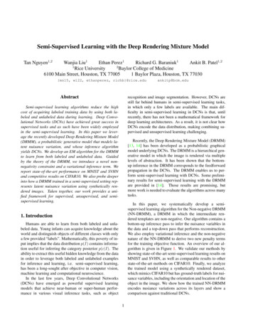
f(x)101055005100ObservationsUnlabeled dataPosterior meanConfidence interval (1 SD)2468hθ (x)510100ObservationsUnlabeled dataPosterior meanConfidence interval (1 SD)2468hθ (x)10Figure 1: Depiction of the variance minimization approach behind semi-supervised deep kernellearning (SSDKL). The x-axis represents one dimension of a neural network embedding and they-axis represents the corresponding output. Left: Without unlabeled data, the model learns anembedding by maximizing the likelihood of labeled data. The black and gray dotted lines show theposterior distribution after conditioning. Right: Embedding learned by SSDKL tries to minimizethe predictive variance of unlabeled data, encouraging unlabeled embeddings to be near labeledembeddings. Observe that the representations of both labeled and unlabeled data are free to change.the strengths of heavily parameterized deep neural networks and nonparametric Gaussianprocesses. While the deep Gaussian process kernel induces structure in an embedding space,the model also allows a priori knowledge of structure (i.e., spatial or temporal) in the inputfeatures to be naturally incorporated through kernel composition. By formalizing the semi-supervised variance minimization objective in the posterior regularization framework, we unify previous semi-supervised approaches such as minimum entropyand minimum variance regularization under a common framework. To our knowledge, thisis the first paper connecting semi-supervised methods to posterior regularization. We demonstrate that SSDKL can use unlabeled data to learn more generalizable featuresand improve performance on a range of regression tasks, outperforming the supervised deepkernel learning method and semi-supervised methods such as virtual adversarial training(VAT) and mean teacher [17, 18]. In a challenging real-world task of predicting povertyfrom satellite images, SSDKL outperforms the state-of-the-art by 15.5%—by incorporatingprior knowledge of spatial structure, the median improvement increases to 17.9%.2PreliminariesWe assume a training set of n labeled examples {(xi , yi )}ni 1 and m unlabeled examples {xj }n mj n 1with instances x Rd and labels y R. Let XL , yL , XU refer to the aggregated features and targets,where XL Rn d , yL Rn , and XU Rm d . At test time, we are given examples XT Rt dthat we would like to predict.There are two major paradigms in semi-supervised learning, inductive and transductive. In inductivesemi-supervised learning, the labeled data (XL , yL ) and unlabeled data XU are used to learn afunction f : X 7 Y that generalizes well and is a good predictor on unseen test examples XT [5].In transductive semi-supervised learning, the unlabeled examples are exactly the test data that wewould like to predict, i.e., XT XU [19]. A transductive learning approach tries to find a functionf : X n m 7 Y n m , with no requirement of generalizing to additional test examples. Although thetheoretical development of SSDKL is general to both the inductive and transductive regimes, weonly test SSDKL in the inductive setting in our experiments for direct comparison against supervisedlearning methods.Gaussian processes A Gaussian process (GP) is a collection of random variables, any finite numberof which form a multivariate Gaussian distribution. Following the notation of [20], a Gaussian processdefines a distribution over functions f : Rd R from inputs to target values. Iff (x) GP (µ(x), kφ (xi , xj ))2
with mean function µ(x) and covariance kernel function kφ (xi , xj ) parameterized by φ, then anycollection of function values is jointly Gaussian,f (X) [f (x1 ), . . . , f (xn )]T N (µ, KX,X ),with mean vector and covariance matrix defined by the GP, s.t. µi µ(xi ) and (KX,X )ij kφ (xi , xj ). In practice, we often assume that observations include i.i.d. Gaussian noise, i.e., y(x) f (x) (x) where N (0, φ2n ), and the covariance function becomesCov(y(xi ), y(xj )) k(xi , xj ) φ2n δijwhere δij I[i j]. To make predictions at unlabeled points XU , we can compute a Gaussianposterior distribution in closed form by conditioning on the observed data (XL , yL ). For a morethorough introduction, we refer readers to [21].Deep kernel learning Deep kernel learning (DKL) combines neural networks with GPs by using aneural network embedding as input to a deep kernel [12]. Given input data x X , a neural networkparameterized by w is used to extract features hw (x) Rp . The outputs are modeled asf (x) GP(µ(hw (x)), kφ (hw (xi ), hw (xj )))for some mean function µ(·) and base kernel function kφ (·, ·) with parameters φ. Parameters θ (w, φ) of the deep kernel are learned jointly by minimizing the negative log likelihood of the labeleddata [20]:Llikelihood (θ) log p(yL XL , θ)(1)For Gaussian distributions, the marginal likelihood is a closed-form, differentiable expression, allowing DKL models to be trained via backpropagation.Posterior regularization In probabilistic models, domain knowledge is generally imposed throughthe specification of priors. These priors, along with the observed data, determine the posteriordistribution through the application of Bayes’ rule. However, it can be difficult to encode ourknowledge in a Bayesian prior. Posterior regularization offers a more direct and flexible mechanismfor controlling the posterior distribution.Let D (XL , yL ) be a collection of observed data. [15] present a regularized optimization formulation called regularized Bayesian inference, or RegBayes. In this framework, the regularized posterioris the solution of the following optimization problem:RegBayes:infq(M D) PprobL(q(M D)) Ω(q(M D))(2)where L(q(M D)) is defined as the KL-divergence between the desired post-data posterior q(M D)over models M and the standard Bayesian posterior p(M D) and Ω(q(M D)) is a posterior regularizer. The goal is to learn a posterior distribution that is not too far from the standard Bayesianposterior while also fulfilling some requirements imposed by the regularization.3Semi-supervised deep kernel learningWe introduce semi-supervised deep kernel learning (SSDKL) for problems where labeled data islimited but unlabeled data is plentiful. To learn from unlabeled data, we observe that a Bayesianapproach provides us with a predictive posterior distribution—i.e., we are able to quantify predictiveuncertainty. Thus, we regularize the posterior by adding an unsupervised loss term that minimizes thepredictive variance at unlabeled data points:1αLlikelihood (θ) Lvariance (θ)nmXLvariance (θ) Var(f (x))Lsemisup (θ) (3)(4)x XUwhere n and m are the numbers of labeled and unlabeled training examples, α is a hyperparametercontrolling the trade-off between supervised and unsupervised components, and θ represents themodel parameters.3
3.1Variance minimization as posterior regularizationOptimizing Lsemisup is equivalent to computing a regularized posterior through solving a specificinstance of the RegBayes optimization problem (2), where our choice of regularizer corresponds tovariance minimization.Let X (XL , XU ) be the observed input data and D (X, yL ) be the input data with labels forthe labeled part XL . Let F denote a space of functions where for f F, f : Rd R maps from theinputs to the target values. Note that here, M (f, θ) is the model in the RegBayes framework, whereθ are the model parameters. We assume that the prior is π(f, θ) and a likelihood density p(D f, θ)exists. Given observed data D, the Bayesian posterior is p(f, θ D), while RegBayes computes adifferent, regularized posterior.Let θ̄ be a specific instance of the model parameters. Instead of maximizing the marginal likelihoodof the labeled training data in a purely supervised approach, we train our model in a semi-supervisedfashion by minimizing the compound objective1α XVarf p (f (x))(5)Lsemisup (θ̄) log p(yL XL , θ̄) nmx XUwhere the variance is with respect to p(f θ̄, D), the Bayesian posterior given θ̄ and D.Theorem 1. Let observed data D, a suitable space of functions F, and parameter space Θ be given.As in [15], we assume that F is a complete separable metric space and Π is an absolutely continuousprobability measure (with respect to background measure η) on (F, B(F)), where B(F) is the Borelσ-algebra, such that a density π exists where dΠ πdη and we have prior density π(f, θ) andlikelihood density p(D f, θ). Then the semi-supervised variance minimization problem (5)inf Lsemisup (θ̄)θ̄is equivalent to the RegBayes optimization problem (2)L(q(f, θ D)) Ω(q(f, θ D))infq(f,θ D) PprobΩ(q(f, θ D)) α0m ZXi 1 p(f θ, D)q(θ D)(f (XU )i Ep [f (XU )i ])2 dη(f, θ) ,f,θwhere α0 αnm , and Pprob {q : q(f, θ D) q(f θ, D)δθ̄ (θ D), θ̄ Θ} is a variational family ofdistributions where q(θ D) is restricted to be a Dirac delta centered on θ̄ Θ.We include a formal derivation in Appendix A.1 and give a brief outline here. It can be shown thatsolving the variational optimization objectiveZinf DKL (q(f, θ D)kπ(f, θ)) q(f, θ D) log p(D f, θ)dη(f, θ)(6)q(f,θ D)f,θis equivalent to minimizing the unconstrained form of the first term L(q(f, θ D)) of the RegBayesobjective in Theorem 1, and the minimizer is precisely the Bayesian posterior p(f, θ D). When werestrict the optimization to q Pprob the solution is of the form q (f, θ D) p(f θ, D)δθ̄ (θ D) forsome θ̄. This allows us to show that (6) is also equivalent to minimizing the first term of Lsemisup (θ̄).Finally, noting that the regularization function Ω only depends on θ̄ (through q(θ D) δθ̄ (θ)), theform of q (f, θ D) is unchanged after adding Ω. Therefore the choice of Ω reduces to minimizingthe predictive variance with respect to q (f θ, D) p(f θ̄, D).Intuition for variance minimization By minimizing Lsemisup , we trade off maximizing thelikelihood of our observations with minimizing the posterior variance on unlabeled data that we wishto predict. The posterior variance acts as a proxy for distance with respect to the kernel functionin the deep feature space, and the regularizer is an inductive bias on the structure of the featurespace. Since the deep kernel parameters are jointly learned, the neural net is encouraged to learn afeature representation in which the unlabeled examples are closer to the labeled examples, therebyreducing the variance on our predictions. If we imagine the labeled data as “supports” for the4
surface representing the posterior mean, we are optimizing for embeddings where unlabeled datatend to cluster around these labeled supports. In contrast, the variance regularizer would not benefitconventional GP learning since fixed kernels would not allow for adapting the relative distancesbetween data points.Another interpretation is that the semi-supervised objective is a regularizer that reduces overfittingto labeled data. The model is discouraged from learning features from labeled data that are not alsouseful for making low-variance predictions at unlabeled data points. In settings where unlabeled dataprovide additional variation beyond labeled examples, this can improve model generalization.Training and inference Semi-supervised deep kernel learning scales well with large amountsof unlabeled data since the unsupervised objective Lvariance naturally decomposes into a sumover conditionally independent terms. This allows for mini-batch training on unlabeled data withstochastic gradient descent. Since all of the labeled examples are interdependent, computing exactgradients for labeled examples requires full batch gradient descent on the labeled data. Therefore,assuming a constant batch size, each iteration of training requires O(n3 ) computations for a Choleskydecomposition, where n is the number of labeled training examples. Performing the GP inferencerequires O(n3 ) one-time cost in the labeled points. However, existing approximation methods basedon kernel interpolation and structured matrices used in DKL can be directly incorporated in SSDKLand would reduce the training complexity to close to linear in labeled dataset size and inference toconstant time per test point [12, 22]. While DKL is designed for the supervised setting where scalingto large labeled datasets is a very practical concern, our focus is on semi-supervised settings wherelabels are limited but unlabeled data is abundant.4Experiments and resultsWe apply SSDKL to a variety of real-world regression tasks in the inductive semi-supervised learningsetting, beginning with eight datasets from the UCI repository [23]. We also explore the challengingtask of predicting local poverty measures from high-resolution satellite imagery [24]. In our reportedresults, we use the squared exponential or radial basis function kernel. We also experimented withpolynomial kernels, but saw generally worse performance. Our SSDKL model is implemented inTensorFlow [25]. Additional training details are provided in Appendix A.3, and code and data forreproducing experimental results can be found on GitHub.24.1BaselinesWe first compare SSDKL to the purely supervised DKL, showing the contribution of unlabeled data.In addition to the supervised DKL method, we compare against semi-supervised methods includingco-training, consistency regularization, generative modeling, and label propagation. Many of thesemethods were originally developed for semi-supervised classification, so we adapt them here forregression. All models, including SSDKL, were trained from random initializations.COREG, or CO-training REGressors, uses two k-nearest neighbor (kNN) regressors, each of whichgenerates labels for the other during the learning process [26]. Unlike traditional co-training, whichrequires splitting features into sufficient and redundant views, COREG achieves regressor diversity byusing different distance metrics for its two regressors [27].Consistency regularization methods aim to make model outputs invariant to local input perturbations[17, 28, 18]. For semi-supervised classification, [29] found that VAT and mean teacher were the bestmethods using fair evaluation guidelines. Virtual adversarial training (VAT) via local distributionalsmoothing (LDS) enforces consistency by training models to be robust to adversarial local inputperturbations [17, 30]. Unlike adversarial training [31], the virtual adversarial perturbation is foundwithout labels, making semi-supervised learning possible. We adapt VAT for regression by choosingthe output distribution N (hθ (x), σ 2 ) for input x, where hθ : Rd R is a parameterized mappingand σ is fixed. Optimizing the likelihood term is then equivalent to minimizing squared error; the LDSterm is the KL-divergence between the model distribution and a perturbed Gaussian (see AppendixA.2). Mean teacher enforces consistency by penalizing deviation from the outputs of a model withthe exponential weighted average of the parameters over SGD iterations [18].2https://github.com/ermongroup/ssdkl5
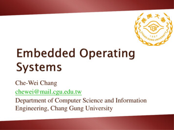
Percent reduction in RMSE compared to DKLn CTsliceBuzzElectricMediann 300NdSSDKLCOREGLabel PropVAEMean TeacherVATSSDKLCOREGLabel PropVAEMean .14Table 1: Percent reduction in RMSE compared to baseline supervised deep kernel learning (DKL)model for semi-supervised deep kernel learning (SSDKL), COREG, label propagation, variational autoencoder (VAE), mean teacher, and virtual adversarial training (VAT) models. Results are averagedacross 10 trials for each UCI regression dataset. Here N is the total number of examples, d is theinput feature dimension, and n is the number of labeled training examples. Final row shows medianpercent reduction in RMSE achieved by using unlabeled data.Label propagation defines a graph structure over the data with edges that define the probabilityfor a categorical label to propagate from one data point to another [32]. If we encode this graphin a transition matrix T and let the current class probabilities be y, then the algorithm iterativelypropagates y T y, row-normalizes y, clamps the labeled data to their known values, and repeatsuntil convergence. We make the extension to regression by letting y be real-valued labels andnormalizing T . As in [32], we use a fully-connected graph and the radial-basis kernel for edgeweights. The kernel scale hyperparameter is chosen using a validation set.Generative models such as the variational autoencoder (VAE) have shown promise in semi-supervisedclassification especially for visual and sequential tasks [33, 34, 35, 36]. We compare against asemi-supervised VAE by first learning an unsupervised embedding of the data and then using theembeddings as input to a supervised multilayer perceptron.4.2UCI regression experimentsWe evaluate SSDKL on eight regression datasets from the UCI repository. For each dataset, we trainon n {50, 100, 200, 300, 400, 500} labeled examples, retain 1000 examples as the hold out test set,and treat the remaining data as unlabeled examples. Following [29], the labeled data is randomly split90-10 into training and validation samples, giving a realistically small validation set. For example,for n 100 labeled examples, we use 90 random examples for training and the remaining 10 forvalidation in every random split. We report test RMSE averaged over 10 trials of random splits tocombat the small data sizes. All kernel hyperparameters are optimized directly through Lsemisup , andwe use the validation set for early stopping to prevent overfitting and for selecting α {0.1, 1, 10}.We did not use approximate GP procedures in our SSDKL or DKL experiments, so the only differenceis the addition of the variance regularizer. For all combinations of input feature dimensions andlabeled data sizes in the UCI experiments, each SSDKL trial (including all training and testing) ranon the order of minutes.Following [20], we choose a neural network with a similar [d-100-50-50-2] architecture and twodimensional embedding. Following [29], we use this same base model for all deep models, includingSSDKL, DKL, VAT, mean teacher, and the VAE encoder, in order to make results comparable acrossmethods. Since label propagation creates a kernel matrix of all data points, we limit the number ofunlabeled examples for label propagation to a maximum of 20000 due to memory constraints. Weinitialize labels in label propagation with a kNN regressor with k 5 to speed up convergence.Table 1 displays the results for n 100 and n 300; full results are included in Appendix A.3.SSDKL gives a 4.20% and 5.81% median RMSE improvement over the supervised DKL in then 100, 300 cases respectively, superior to other semi-supervised methods adapted for regression.A Wilcoxon signed-rank test versus DKL shows significance at the p 0.05 level for at least onelabeled training set size for all 8 datasets.The same learning rates and initializations are used across all UCI datasets for SSDKL. We uselearning rates of 1 10 3 and 0.1 for the neural network and GP parameters respectively and6
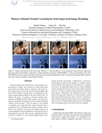
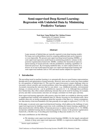
Figure 2: Left: Average test RMSE vs. number of labeled examples for UCI Elevators dataset,n {50, 100, 200, 300, 400, 500}. SSDKL generally outperforms supervised DKL, co-trainingregressors (COREG), and virtual adversarial training (VAT). Right: SSDKL performance on povertyprediction (Section 4.3) as a function of α, which controls the trade-off between labeled and unlabeledobjectives, for n 300. The dotted lines plot the performance of DKL and COREG. All resultsaveraged over 10 trials. In both panels, shading represents one standard deviation.initialize all GP parameters to 1. In Fig. 2 (right), we study the effect of varying α to trade offbetween maximizing the likelihood of labeled data and minimizing the variance of unlabeled data. Alarge α emphasizes minimization of the predictive variance while a small α focuses on fitting labeleddata. SSDKL improves on DKL for values of α between 0.1 and 10.0, indicating that performanceis not overly reliant on the choice of this hyperparameter. Fig. 2 (left) compares SSDKL to purelysupervised DKL, COREG, and VAT as we vary the labeled training set size. For the Elevators dataset,DKL is able to close the gap on SSDKL as it gains access to more labeled data. Relative to the othermethods, which require more data to fit neural network parameters, COREG performs well in thelow-data regime.Surprisingly, COREG outperformed SSDKL on the Blog, CTslice, and Buzz datasets. We found thatthese datasets happen to be better-suited for nearest neighbors-based methods such as COREG. AkNN regressor using only the labeled data outperformed DKL on two of three datasets for n 100,beat SSDKL on all three for n 100, beat DKL on two of three for n 300, and beat SSDKL onone of three for n 300. Thus, the kNN regressor is often already outperforming SSDKL with onlylabeled data—it is unsurprising that SSDKL is unable to close the gap on a semi-supervised nearestneighbors method like COREG.Representation learning To gain some intuition about how the unlabeled data helps in the learningprocess, we visualize the neural network embeddings learned by the DKL and SSDKL models on theSkillcraft dataset. In Fig. 3 (left), we first train DKL on n 100 labeled training examples and plotthe two-dimensional neural network embedding that is learned. In Fig. 3 (right), we train SSDKLon n 100 labeled training examples along with m 1000 additional unlabeled data points andplot the resulting embedding. In the left panel, DKL learns a poor embedding—different colorsrepresenting different output magnitudes are intermingled. In the right panel, SSDKL is able to usethe unlabeled data for regularization, and learns a better representation of the dataset.4.3Poverty predictionHigh-resolution satellite imagery offers the potential for cheap, scalable, and accurate tracking ofchanging socioeconomic indicators. In this task, we predict local poverty measures from satelliteimages using limited amounts of poverty labels. As described in [2], the dataset consists of 3, 066villages across five Africa countries: Nigeria, Tanzania, Uganda, Malawi, and Rwanda. These includesome of the poorest countries in the world (Malawi and Rwanda) as well as some that are relativelybetter off (Nigeria), making for a challenging and realistically diverse problem.7
Figure 3: Left: Two-dimensional embeddings learned by supervised deep kernel learning (DKL)model on the Skillcraft dataset using n 100 labeled training examples. The colorbar shows themagnitude of the normalized outputs. Right: Embeddings learned by semi-supervised deep kernellearning (SSDKL) model using n 100 labeled examples plus an additional m 1000 unlabeledexamples. By using unlabeled data for regularization, SSDKL learns a better representation.Percent reduction in RMSE (n 300)CountrySpatial 1.3Median17.915.513.8Table 2: Percent RMSE reduction in a poverty measure prediction task compared to baseline ridgeregression model used in [2]. SSDKL and DKL models use only satellite image data. Spatial SSDKLincorporates both location and image data through kernel composition. Final row shows medianRMSE reduction of each model averaged over 10 trials.In this experiment, we use n 300 labeled satellite images for training. With such a small dataset,we can not expect to train a deep convolutional neural network (CNN) from scratch. Instead we takea transfer learning approach as in [24], extracting 4096-dimensional visual features and using theseas input. More details are provided in Appendix A.5.Incorporating spatial information In order to highlight the usefulness of kernel composition, weexplore extending SSDKL with a spatial kernel. Spatial SSDKL composes two kernels by summingan image feature kernel and a separate location kernel that operates on location coordinates (lat/lon).By treating them separately, it explicitly encodes the knowledge that location coordinates are spatiallystructured and distinct from image features.As shown in Table 2, all models outperform the baseline state-of-the-art ridge regression model from[2]. Spatial SSDKL significantly outperforms the DKL and SSDKL models that use only imagefeatures. Spatial SSDKL outperforms the other models by directly modeling location coordinatesas spatial features, showing that kernel composition can effectively incorporate prior knowledge ofstructure.5Related work[37] introduced deep Gaussian processes, which stack GPs in a hierarchy by modeling the outputs ofone layer with a Gaussian process in the next layer. Despite the suggestive name, these models do notintegrate deep neural networks and Gaussian processes.8
[12] proposed deep kernel learning, combining neural networks with the non-parametric flexibilityof GPs and training end-to-end in a fully supervised setting. Extensions have explored approximateinference, stochastic gradient training, and recurrent deep kernels for sequential data [22, 38, 39].Our method draws inspiration from transductive experimental design, which chooses the mostinformative points (experiments) to measure by seeking data points that are both hard to predict andinformative for the unexplored test data [40]. Similar prediction uncertainty approaches have beenexplored in semi-supervised classification models, such as minimum entropy and minimum varianceregularization, which can now also be understood in the posterior regularization framework [7, 41].Recent work in generative adversarial networks (GANs) [33], variational autoencoders (VAEs) [34],and other generative models have achieved promising results on various semi-supervised classificationtasks [35, 36]. However, we find that these models are not as well-suited for generic regression taskssuch as in the UCI repository as for audio-visual tasks.Consistency regularization posits that the model’s output should be invariant to reasonable perturbations of the input [17, 28, 18]. Combining adversarial training [31] with consistency regularization,virtual adversarial training uses a label-free regularization term that allows for semi-supervisedtraining [17]. Mean teacher adds a regularization term that penalizes deviation from a exponentialweighted average of the parameters over SGD iterations [18]. For semi-s
3 Semi-supervised deep kernel learning We introduce semi-supervised deep kernel learning (SSDKL) for problems where labeled data is limited but unlabeled data is plentiful. To learn from unlabeled data, we observe that a Bayesian approach provides us with a predictive posterior distribution—i.e., we are able to quantify predictive uncertainty.