Transcription
Data MiningDimensionality reductionHamid BeigySharif University of TechnologyFall 1395Hamid Beigy (Sharif University of Technology)Data MiningFall 13951 / 42
Outline1Introduction2Feature selection methods3Feature extraction methodsPrincipal component analysisKernel principal component analysisFactor analysisLocally Linear EmbeddingLinear discriminant analysisHamid Beigy (Sharif University of Technology)Data MiningFall 13952 / 42
Table of contents1Introduction2Feature selection methods3Feature extraction methodsPrincipal component analysisKernel principal component analysisFactor analysisLocally Linear EmbeddingLinear discriminant analysisHamid Beigy (Sharif University of Technology)Data MiningFall 13953 / 42
IntroductionThe complexity of any classifier or regressors depends on the number of input variables orfeatures. These complexities includeTime complexity: In most learning algorithms, the time complexity depends on thenumber of input dimensions(D) as well as on the size of training set (N). Decreasing Ddecreases the time complexity of algorithm for both training and testing phases.Space complexity: Decreasing D also decreases the memory amount needed for trainingand testing phases.Samples complexity: Usually the number of training examples (N) is a function of lengthof feature vectors (D). Hence, decreasing the number of features also decreases thenumber of training examples.Usually the number of training pattern must be 10 to 20 times of the number of features.Hamid Beigy (Sharif University of Technology)Data MiningFall 13953 / 42
IntroductionThere are several reasons why we are interested in reducing dimensionality as a separatepreprocessing step.Decreasing the time complexity of classifiers or regressors.Decreasing the cost of extracting/producing unnecessary features.Simpler models are more robust on small data sets. Simpler models have less varianceand thus are less depending on noise and outliers.Description of classifier or regressors is simpler / shorter.Visualization of data is simpler.Hamid Beigy (Sharif University of Technology)Data MiningFall 13954 / 42
Peaking phenomenonIn practice, for a finite number of training examples (N), by increasing the number offeatures (l) we obtain an initial improvement in performance, but after a critical value,further increase of the number of features results in an increase of the probability of error.This phenomenon is also known as the peaking phenomenon.If the number of samples increases (N2 N1 ), the peaking phenomenon occures forlarger number of features (l2 l1 ).Hamid Beigy (Sharif University of Technology)Data MiningFall 13955 / 42
Dimensionality reduction methodsThere are two main methods for reducing the dimensionality of inputsFeature selection: These methods select d (d D) dimensions out of D dimensions andD d other dimensions are discarded.Feature extraction: Find a new set of d (d D) dimensions that are combinations of theoriginal dimensions.Hamid Beigy (Sharif University of Technology)Data MiningFall 13956 / 42
Table of contents1Introduction2Feature selection methods3Feature extraction methodsPrincipal component analysisKernel principal component analysisFactor analysisLocally Linear EmbeddingLinear discriminant analysisHamid Beigy (Sharif University of Technology)Data MiningFall 13957 / 42
Feature selection methodsFeature selection methods select d (d D) dimensions out of D dimensions and D dother dimensions are discarded.Reasons for performing feature selectionIncreasing the predictive accuracy of classifiers or regressors.Removing irrelevant features.Enhancing learning efficiency (reducing computational and storage requirements).Reducing the cost of future data collection (making measurements on only those variablesrelevant for discrimination/prediction).Reducing complexity of the resulting classifiers/regressors description (providing an improvedunderstanding of the data and the model).Feature selection is not necessarily required as a pre-processing step for classification/regression algorithms to perform well.Several algorithms employ regularization techniques to handle over-fitting or averagingsuch as ensemble methods.Hamid Beigy (Sharif University of Technology)Data MiningFall 13957 / 42
Feature selection methodsFeature selection methods can be categorized into three categories.Filter methods: These methods use the statistical properties of features to filter out poorlyinformative features.Wrapper methods: These methods evaluate the feature subset within classifier/regressoralgorithms. These methods are classifier/regressors dependent and have better performancethan filter methods.Embedded methods:These methods use the search for the optimal subset intoclassifier/regression design. These methods are classifier/regressors dependent.Two key steps in feature selection process.Evaluation: An evaluation measure is a means of assessing a candidate feature subset.Subset generation: A subset generation method is a means of generating a subset forevaluation.Hamid Beigy (Sharif University of Technology)Data MiningFall 13958 / 42
Feature selection methods (Evaluation measures)Large number of features are not informative- either irrelevant or redundant.Irrelevant features are those features that don’t contribute to a classification or regressionrule.Redundant features are those features that are strongly correlated.In order to choose a good feature set, we require a means of a measure to contribute tothe separation of classes, either individually or in the context of already selected features.We need to measure relevancy and redundancy.There are two types of measuresMeasures that relay on the general properties of the data. These assess the relevancy ofindividual features and are used to eliminate feature redundancy. All these measures areindependent of the final classifier. These measures are inexpensive to implement but may notwell detect the redundancy.Measures that use a classification rule as a part of their evaluation. In this approach, aclassifier is designed using the reduced feature set and a measure of classifier performance isemployed to assess the selected features. A widely used measure is the error rate.Hamid Beigy (Sharif University of Technology)Data MiningFall 13959 / 42
Feature selection methods (Evaluation measures)The following measures relay on the general properties of the data.Feature ranking: Features are ranked by a metric and those that fail to achieve a prescribedscore are eliminated.Examples of these metrics are: Pearson correlation, mutual information, and information gain.Interclass distance: A measure of distance between classes is defined based on distancesbetween members of each class.Example of these metrics is: Euclidean distance.Probabilistic distance: This is the computation of a probabilistic distance betweenclass-conditional probability density functions, i.e. the distance between p(x C1 ) and p(x C2 )(two-classes).Example of these metrics is: Chhernoff dissimilarity measure.Probabilistic dependency: These measures are multi-class criteria that measure the distancebetween class-conditional probability density functions and the mixture probability densityfunction for the data irrespective of the class, i.e. the distance between p(x Ci ) and p(x).Example of these metrics is: Joshi dissimilarity measure.Hamid Beigy (Sharif University of Technology)Data MiningFall 139510 / 42
Feature selection methods (Search algorithms)Complete search: These methods guarantee to find the optimal subset of featuresaccording to some specified evaluation criteria.For example exhaustive search and branch and bound methods are complete.Sequential search: In these methods, features are added or removed sequentially. Thesemethods are not optimal, but are simple to implement and fast to produce results.Best individual N: The simplest method is to assign a score to each feature and thenselect N top ranks features.Sequential forward selection: It is a bottom-up search procedure that adds new featuresto a feature set one at a time until the final feature set is reached.Generalized sequential forward selection: In this approach, at each time r 1, featuresare added instead of a single feature.Sequential backward elimination: It is a top-down procedure that deletes a single featureat a time until the final feature set is reached.Generalized sequential backward elimination : In this approach, at each time r 1features are deleted instead of a single feature.Hamid Beigy (Sharif University of Technology)Data MiningFall 139511 / 42
Table of contents1Introduction2Feature selection methods3Feature extraction methodsPrincipal component analysisKernel principal component analysisFactor analysisLocally Linear EmbeddingLinear discriminant analysisHamid Beigy (Sharif University of Technology)Data MiningFall 139512 / 42
Feature extractionIn feature extraction, we are interested to find a new set of k (k D) dimensions thatare combinations of the original D dimensions.Feature extraction methods may be supervised or unsupervised.Examples of feature extraction methodsPrincipal component analysis (PCA)Factor analysis (FA)sMulti-dimensional scaling (MDS)ISOMapLocally linear embeddingLinear discriminant analysis (LDA)Hamid Beigy (Sharif University of Technology)Data MiningFall 139512 / 42
Principal component analysisPCA project D dimensional input vectors to k dimensional input vectors via a linearmapping with minimum loss of information. Dimensions are combinations of the originalD dimensions.The problem is to find a matrix W such that the following mapping results in theminimum loss of information.Z WTXPCA is unsupervised and tries to maximize the variance.The principle component is w1 such that the sample after projection onto w1 is mostspread out so that the difference between the sample points becomes most apparent.For uniqueness of the solution, we require kw1 k 1,Let Σ Cov (X ) and consider the principle component w1 , we havez1 w1T xVar (z1 ) E [(w1T x w1T µ)2 ] E [(w1T x w1T µ)(w1T x w1T µ)] E [w1T (x µ)(x µ)T w1 ] w1T E [(x µ)(x µ)T ]w1 w1T Σw1Hamid Beigy (Sharif University of Technology)Data MiningFall 139513 / 42
Principal component analysis (cont.)The mapping problem becomesw1 argmax w T Σwwsubject to w1T w1 1.Writing this as Lagrange problem, we havemaximize w1T Σw1 α(w1T w1 1)w1Taking derivative with respect to w1 and setting it equal to 0, we obtain2Σw1 2αw1 Σw1 αw1Hence w1 is eigenvector of Σ and α is the corresponding eigenvalue.Since we want to maximize Var (z1 ), we haveVar (z1 ) w1T Σw1 αw1T w1 αHence, we choose the eigenvector with the largest eigenvalue, i.e. λ1 α.Hamid Beigy (Sharif University of Technology)Data MiningFall 139514 / 42
Principal component analysis (cont.)The second principal component, w2 , should alsomaximize variancebe unit lengthorthogonal to w1 (z1 and z2 must be uncorrelated)The mapping problem for the second principal component becomesw2 argmax w T Σwwsubject to w2T w2 1 and w2T w1 0.Writing this as Lagrange problem, we havemaximize w2T Σw2 α(w2T w2 1) β(w2T w1 0)w2Taking derivative with respect to w2 and setting it equal to 0, we obtain2Σw2 2αw2 βw1 0Pre-multiply by w1T , we obtain2w1T Σw2 2αw1T w2 βw1T w1 0Note that w1T w2 0 and w1T Σw2 (w2T Σw1 )T w2T Σw1 is a scaler.Hamid Beigy (Sharif University of Technology)Data MiningFall 139515 / 42
Principal component analysis (cont.)Since Σw1 λ1 w1 , therefore we havew1T Σw2 w2T Σw1 λ1 w2T w1 0Then β 0 and the problem reduces toΣw2 αw2This implies that w2 should be the eigenvector of Σ with the second largest eigenvalueλ2 α.Similarly, you can show that the other dimensions are given by the eigenvectors withdecreasing eigenvalues.Since Σ is symmetric, for two different eigenvalues, their corresponding eigenvectors areorthogonal. (Show it)If Σ is positive definite (x T Σx 0 for all non-null vector x), then all its eigenvalues arepositive.If Σ is singular, its rank is k (k D) and λi 0 for i k 1, . . . , D.Hamid Beigy (Sharif University of Technology)Data MiningFall 139516 / 42
Principal component analysis (cont.)DefineZ W T (X m)Then k columns of W are the k leading eigenvectors of S (the estimator of Σ).m is the sample mean of X .Subtracting m from X before projection centers the data on the origin.How to normalize variances?Hamid Beigy (Sharif University of Technology)Data MiningFall 139517 / 42
Principal component analysis (cont.)How to select k?QIf all eigenvalues are positive and S Di 1 λi is small, then some eigenvalues have littlecontribution to the variance and may be discarded.Scree graph is the plot of variance as a function of the number of eigenvectors.Hamid Beigy (Sharif University of Technology)Data MiningFall 139518 / 42
Principal component analysis (cont.)How to select k?We select the leading k components that explain more than for example 95% of thevariance.The proportion of variance (POV) isPkλiPOV Pi 1Di 1 λiBy visually analyzing it, we can choose k.Hamid Beigy (Sharif University of Technology)Data MiningFall 139519 / 42
Principal component analysis (cont.)How to select k?Another possibility is to ignore the eigenvectors whose corresponding eigenvalues are lessthan the average input variance (why?).In the pre-processing phase, it is better to pre-process data such that each dimension hasmean 0 and unit variance(why and when?).Question: Can we use the correlation matrix instead of covariance matrix? Drive solutionfor PCA.Hamid Beigy (Sharif University of Technology)Data MiningFall 139520 / 42
Principal component analysis (cont.)PCA is sensitive to outliers. A few points far from the center have large effect on thevariances and thus eigenvectors.Question: How can use the robust estimation methods for calculating parameters in thepresence of outliers?A simple method is discarding the isolated data points that are far away.Question: When D is large, calculating, sorting, and processing of S may be tedious. Is itpossible to calculate eigenvectors and eigenvalues directly from data without explicitlycalculating the covariance matrix?Hamid Beigy (Sharif University of Technology)Data MiningFall 139521 / 42
Principal component analysis (reconstruction error)In PCA, input vector x is projected to the z space asz W T (x µ)When W is an orthogonal matrix (W T W I ), it can be back-projected to the originalspace asx̂ Wz µx̂ is the reconstruction of x from its representation in the z space.Question: Show that PCA minimizes the following reconstruction error.Xkx̂i xi k2iThe reconstruction error depends on how many of the leading components are taken intoaccount.Hamid Beigy (Sharif University of Technology)Data MiningFall 139522 / 42
Kernel principal component analysisPCA can be extended to find nonlinear directions in the data using kernel methods.Kernel PCA finds the directions of most variance in the feature space instead of the inputspace.Linear principal components in the feature space correspond to nonlinear directions in theinput space.Using kernel trick, all operations can be carried out in terms of the kernel function ininput space without having to transform the data into feature space.Let φ correspond to a mapping from the input space to the feature space.Each point in feature space is given as the image of φ(x) of the point x in the input space.In feature space, we can find the first kernek principal component W1 (W1T W1 1) bysolvingΣφ W1 λ 1 W1Covariance matrix Σφ in feature space is equal toΣφ N1 Xφ(xi )φ(xi )TNi 1We assume that the points are centered.Hamid Beigy (Sharif University of Technology)Data MiningFall 139523 / 42
Kernel principal component analysis (cont.)Plugging Σφ into Σφ W1 λ1 W1 , we obtainN1 Xφ(xi )φ(xi )TN1N!W1 λ 1 W1i 1NX φ(xi ) φ(xi )T W1 λ 1 W1i 1 N Xφ(xi )T W1i 1Nλ1NXφ(xi ) W1ci φ(xi ) W1i 1ci φ(xi )T W1Nλ1is a scalar valueHamid Beigy (Sharif University of Technology)Data MiningFall 139524 / 42
Kernel principal component analysis (cont.)Now substitutePNi 1 ci φ(xi ) W1 in Σφ W1 λ1 W1 , we obtainN1 Xφ(xi )φ(xi )TN!i 1NX!ci φ(xi ) λ1i 1NXci φ(xi )i 1NXN N1 XXcj φ(xi )φ(xi )T φ(xj ) λ1ci φ(xi )Ni 1 j 1i 1 NNNXXX φ(xi )cj φ(xi )T φ(xj ) Nλ1ci φ(xi )i 1j 1i 1Replacing φ(xi )T φ(xj ) by K (xi , xj )NXi 1Hamid Beigy (Sharif University of Technology) φ(xi )NX cj K (xi , xj ) Nλ1NXci φ(xi )i 1j 1Data MiningFall 139525 / 42
Kernel principal component analysis (cont.)Multiplying with φ(xk )T , we obtainNX φ(xk )T φ(xi )i 1NX cj K (xi , xj ) Nλ1j 1NX K (xk , xi )i 1NXNXci φ(xk )T φ(xi )i 1 cj K (xi , xj ) Nλ1j 1NXci K (xk , xj )i 1By some algebraic simplificatin, we obtain (do it)K 2C Nλ1 KCMultiplying by K 1 , we obtainKC Nλ1 CKC η1 CWeight vector C is the eigenvector corresponding to the largest eigenvalue η1 of thekernel matrix K .Hamid Beigy (Sharif University of Technology)Data MiningFall 139526 / 42
Kernel principal component analysis (cont.)ReplacingPNi 1 ci φ(xi ) W1 in constraint W1T W1 1, we obtainN XNXcj cj φ(xi )T φ(xj ) 1i 1 j 1C T KC 1Using KC η1 C , we obtainC T (η1 C ) 1η1 C T C 11 C 2 η1Since C is an eigenvector of K , it will have unit norm.qTo ensure that W1 is a unit vector, multiply C by η11Hamid Beigy (Sharif University of Technology)Data MiningFall 139527 / 42
Kernel principal component analysis (cont.)In general, we do not map input space to the feature space via φ, hence we cannotcompute W1 usingNXci φ(xi ) W1i 1We can project any point φ(x) on to principal direction W1W1T φ(x) NXTci φ(xi ) φ(x) i 1NXci K (xi , x)i 1When x xi is one of the input points, we haveai W1T φ(xi ) KiT Cwhere Ki is the column vector corresponding to the I th row of K and ai is the vector inthe reduced dimension.This shows that all computation are carried out using only kernel operations.Hamid Beigy (Sharif University of Technology)Data MiningFall 139528 / 42
Factor analysisIn PCA, from the original dimensions xi (for i 1, . . . , D), we form a new set of variablesz that are linear combinations of xiZ W T (X µ)In factor analysis (FA), we assume that there is a set of unobservable, latent factors zj(for j 1, . . . , k), which when acting in combination generate x.Thus the direction is opposite that of PCA.The goal is to characterize the dependency among the observed variables by means of asmaller number of factors.Suppose there is a group of variables that have high correlation among themselves andlow correlation with all the other variables. Then there may be a single underlying factorthat gave rise to these variables.FA, like PCA, is a one-group procedure and is unsupervised. The aim is to model the datain a smaller dimensional space without loss of information.In FA, this is measured as the correlation between variables.Hamid Beigy (Sharif University of Technology)Data MiningFall 139529 / 42
Factor analysis (cont.)Hamid Beigy (Sharif University of Technology)Data MiningFall 139530 / 42
Factor analysis (cont.)As in PCA, we have a sample x drawn from some unknown probability density withE [x] µ and Cov (x) Σ.We assume that the factors are unit normals, E [zj ] 0, Var (zj ) 1, and areuncorrelated,Cov (zi , zj ) 0, i 6 j.To explain what is not explained by the factors, there is an added source for each inputwhich we denote by i .It is assumed to be zero-mean, E [ i ] 0, and have some unknown variance, Var ( i ) ψi.These specific sources are uncorrelated among themselves, Cov ( i , i ) 0, i 6 j, and arealso uncorrelated with the factors, Cov ( i , zj ) 0, i, j.FA assumes that each input dimension, xi can be written as a weighted sum of k Dfactors, zj plus the residual term.xi µi vi1 z1 vi2 z2 . . . vik zk iThis can be written in vector-matrix form asx µ VZ iV is the D k matrix of weights, called factor loadings.Hamid Beigy (Sharif University of Technology)Data MiningFall 139531 / 42
Factor analysis (cont.)We assume that µ 0 and we can always add µ after projection.Given that Var (zj ) 1 and Var ( i ) ψi and22Var (xi ) vi1 vi2 . . . vik2 ψiIn vector-matrix form, we haveΣ Var (X ) VV T ΨThere are two uses of factor analysis:It can be used for knowledge extraction when we find the loadings and try to express thevariables using fewer factors.It can also be used for dimensionality reduction when k D.Hamid Beigy (Sharif University of Technology)Data MiningFall 139532 / 42
Factor analysis (cont.)For dimensionality reduction, we need to find the factor, zj , from xi .We want to find the loadings wji such thatzj DXwji xi ii 1In vector form, for input x, this can be written asz WTx For N input, the problem is reduced to linear regression and its solution isW (X T X ) 1 X T ZWe do not know Z ; We multiply and divide both sides by N 1 and obtain (drive it!)T 1W (N 1)(X X )XTZ N 1 XTXN 1 1XTZ S 1 VN 1Z XW XS 1 VHamid Beigy (Sharif University of Technology)Data MiningFall 139533 / 42
Locally Linear EmbeddingLocally linear embedding (LLE) recovers global nonlinear structure from locally linear fits.The idea is that each point can be approximated as a weighted sum of its neighbors.The neighbors either defined using a given number of neighbors (n) or distance threshold( ).Let x r be an example in the input space and its neighbors be x(rs ) . We find weights insuch a way that minimize the following objective function.E [W x] NX2rx r 1Xwrs x(rs )sThe idea in LLE is that the reconstruction weights wrs reflect the intrinsic geometricproperties of the data is also valid for the new space.The first step of LLEPis to find wrs in such a way that minimize the above objectivefunction subject to s wrs 1.Hamid Beigy (Sharif University of Technology)Data MiningFall 139534 / 42
Locally Linear Embedding (cont.)The second step of LLE is to keep wrs fixed and construct the new coordinates Y in sucha way that minimize the following objective function.REPORTSstraints: first, thattructed only fromWij ! 0 if X!j doesE [Y W ] not belong to the set of neighbors of X!i;second, that the rows of the weight matrixsum to one: "jWij ! 1. The optimal weightsin such a way that Cov (Y ) IHamid Beigy (Sharif University of Technology)NX2ry Xwrs y(rs )(6) are foundWij subjectsr 1to these constraintsby solving a least-squares problem (7).constrained weights that minimizeandtheseEThe[Y] 0. errors obey an importantreconstructionsymmetry: for any particular data point, theyare invariant to rotations, rescalings, andtranslations of that data point and its neighbors. By symmetry, it follows that the reconstruction weights characterize intrinsic geometric properties of each neighborhood, asopposed to properties that depend on a particular frame of reference (8). Note that theinvariance to translations is specifically enforced by the sum-to-one constraint on theS. T. Roweis and L. K. Saul, ”Nonlinearrows of the weight matrix.Suppose the data lieDimensionalityon or near a smoothReduction by Locallynonlinear manifold of lower dimensionality dLinear then,Embedding”,SCIENCE, VOL 290,## D. To a good approximationthereexists a linear mapping— consisting of aNo.22,pp.2323-2326,Dec. 2000.translation, rotation, and rescaling—thatmaps the high-dimensional coordinates ofeach neighborhood to global internal coordinates on the manifold. By design, the reconstruction weights Wij reflect intrinsic geometric properties of the data that are invariant toexactly such transformations. We thereforeexpect their characterization of local geometry in the original data space to be equallyvalid for local patches on the manifold. Inparticular,same weights Wij that reconData theMiningFall 139535 / 42
Linear discriminant analysisLinear discriminant analysis (LDA) is a supervised method for dimensionality reduction forclassification problems.Consider first the case of two classes, and suppose we take the D dimensional inputvector x and project it down to one dimension usingz WTxIf we place a threshold on z and classify z w0 as class C1 , and otherwise class C2 , thenwe obtain our standard linear classifier.In general, the projection onto one dimension leads to a considerable loss of information,and classes that are well separated in the original D dimensional space may becomestrongly overlapping in one dimension.Hamid Beigy (Sharif University of Technology)Data MiningFall 139536 / 42
Linear discriminant analysis(cont.)However, by adjusting the components of the weight vector W , we can select a projectionthat maximizes the class separation.Consider a two-class problem in which there are N1 points of class C1 and N2 points ofclass C2 , so that the mean vectors of the two classes are given bymj 1 XxiNji CjHamid Beigy (Sharif University of Technology)Data MiningFall 139537 / 42
Linear discriminant analysis (cont.)xx112Introduction to Pattern AnalysisRicardo Gutierrez-OsunaThe simplestTexasmeasureA&M University of the separation of the classes, when projected onto W , is theLinearAnalysis, two-classes (2)separation of theDiscriminantprojected class means.This !suggeststhatmightchooseW so asvector,to maximizeIn orderto wefinda goodprojectionwe need to define a measureTof separation betweenmtheprojections2 m1 W (m2 m1 )where!The mean vector of each class in x and y feature space isµi !1NiT1 ! 1mandj µW"x m" jy ! N " wNix#!ii y#!ii x#!iTx ! w TµiThis expression can be made arbitrarily large simply by increasing the magnitudeP 2 of W .We could then choose the distance between the projected means as our objectiveTo solve this nctioni wi 1.T Using a Lagrange multiplier to performwe then find that%J( w ) !theµ1 &constrainedµ2 ! w µ1 & µ2maximization,!!W (m2 m1 )However, the distance between the projected means is not a very good measure since itdoes not take into account the standard deviation within the classesx2'1This axis yields better class separability'2x1This axis has a larger distance between meansIntroduction to Pattern AnalysisHamid Beigy (Sharif UniversityTechnology)Ricardo ofGutierrez-Osuna3Data MiningFall 139538 / 42
Linear discriminant analysis (cont.)This approach has a problem: The following figure shows two classes that are wellseparated in the original two dimensional space but that have considerable overlap whenprojected onto the line joining their means.This difficulty arises from the strongly non-diagonal covariances of the class distributions.The idea proposed by Fisher is to maximize a function that will give a large separationbetween the projected class means while also giving a small variance within each class,thereby minimizing the class overlap.Hamid Beigy (Sharif University of Technology)Data MiningFall 139539 / 42
Linear discriminant analysis (cont.)The idea proposed by Fisher is to maximize a function that will give a large separationbetween the projected class means while also giving a small variance within each class,thereby minimizing the class overlap.The projection z W T x transforms the set of labeled data points in x into a labeled setin the one-dimensional space z.The within-class variance of the transformed data from class Cj equalsXsj2 (zi mj )2i Cjwherezi w T xi .We can define the total within-class variance for the whole data set to be s12 s22 . .The Fisher criterion is defined to be the ratio of the between-class variance to thewithin-class variance and is given byJ(W ) Hamid Beigy (Sharif University of Technology)(m2 m1 )2s12 s22Data MiningFall 139540 / 42
Linear discriminant analysis (cont.)Between-class covariance matrix equals toSB (m2 m1 )(m2 m1 )TTotal within-class covariance matrix equals toXXSW (xi m1 ) (xi m1 )T (xi m2 ) (xi m2 )Ti C1i C2J(W ) can be written asJ(w ) W T SB WW T SW WTo maximize J(W ), we differentiate with respect to W and we obtain W T SB W SW W W T SW W SB WSB W is always in the direction of (m2 m1 ) (Show it!).We can drop the scalar factors W T SB W and W T SW W (why?).Multiplying both sides of S 1W we then obtain (Show it!)W S 1W (m2 m1 )Hamid Beigy (Sharif University of Technology)Data MiningFall 139541 / 42
Linear discriminant analysis (cont.)The result W S 1W (m2 m1 ) is known as Fisher’s linear discriminant, although strictlyit is not a discriminant but rather a specific choice of direction for projection of the datadown to one dimension.The projected data can subsequently be used to construct a discriminant function.The above idea can be extended to multiple classes (Read section 4.1.6 of Bishop).How the Fisher’s linear discriminant can be used for dimensionality reduction? (Show it!)Hamid Beigy (Sharif University of Technology)Data MiningFall 139542 / 42
Wrapper methods:These methods evaluate the feature subset within classi er/regressor algorithms. These methods are classi er/regressors dependent and have better performance than lter methods. Embedded methods:These methods use the search for the optimal subset into classi er/regression design. These methods are classi er/regressors dependent.