Transcription
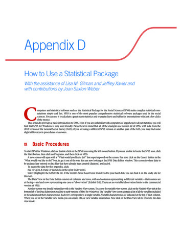
Appendix DHow to Use a Statistical PackageWith the assistance of Lisa M. Gilman and Jeffrey Xavier andwith contributions by Joan Saxton WeberComputers and statistical software such as the Statistical Package for the Social Sciences (SPSS) make complex statistical computations simple and fast. SPSS is one of the most popular comprehensive statistical software packages used in the socialsciences. You can use it to calculate a great many statistics and to create charts and tables for presentations with just a few clicksof the mouse.This appendix provides a basic introduction to SPSS. Even if you are unfamiliar with computers or apprehensive about statistics, you willfind that SPSS for Windows is very user friendly. Please bear in mind that all of the examples use version 22 of SPSS, with data from the2012 version of the General Social Survey (GSS); if you are using a different SPSS version or another year of the GSS, you may find someslight differences in procedures or answers.2 Basic ProceduresTo start SPSS for Windows, click or double-click on the SPSS icon using the left mouse button. If you are unable to locate the SPSS icon, clickthe Start button, then click on Programs, and then click on SPSS.A new screen will open with a “What would you like to do?” box superimposed on the screen. For now, click on the Cancel button in the“What would you like to do?” box, to get it out of the way. You are now looking at the SPSS Data Editor window. This screen is where data tobe analyzed are entered or data files that have already been created (datasets) are loaded.To access the data for this appendix, click:File Æ Open Æ Data (or just click on the open folder icon).Select (highlight) the GSS2012x file. If the GSS2012x file hasn’t been transferred to your hard disk, you can find it on the study site forthis text.The Data View in the Data Editor consists of columns and rows, with each column representing a different variable—their names areat the top—and each row representing one case or “observation” (Exhibit D.1). There are no variable/observation limits in the commercialversion of SPSS.Another screen you should be familiar with is the Variable View screen. To access the variable view screen, click on the Variable View tab at thebottom left of the Data Editor (not available in early versions of SPSS for Windows). The Variable View screen contains a list of all the variables includedin the dataset and their characteristics. Each row corresponds to a single variable. Variable characteristics are indicated at the top of each column.When you are in the Variable View mode, you can create, edit, or view variable information. Now click on the Data View tab to return to the dataview mode.
Exhibit D.1Launching a Research ProjectLooking at the DataThere are several ways to learn more about the variables and numbers that you see in the Data View screen. The names of the variablesare listed across the top of the screen. You can also see the list of variables in the GSS2012x file by clicking on the variable list icon atthe top of the Data Editor screen. When you click on any variable in the resulting window, you can see the details that show how it wascoded. But the easiest way to learn about the variables in the dataset is to switch from the Data View to the Variable View screen byclicking on the tab in the lower left.You can tell what some variables are just by their SPSS variable names, like SEX. However, many variables are responses tospecific questions and we can’t tell just what they are on the basis of the shorthand variable name. Instead, we can inspect thevariable label in the “Label” column corresponding to that variable in the Variable View screen (you may need to widen theLabel column by dragging the separator line at the top of the column with your mouse).SPSS understands numbers much better than text, so all the answers to each GSS question have been coded. This means that, forevery variable, each response category has been assigned a numerical value. For some variables, such as AGE and EDUC, the numberyou see is simply the number of years. For other variables, such as SEX and RACED, each number corresponds to a particular responsecategory. For example, go to the Variable View screen and click on the “Values” cell in the row corresponding to the variable SEX. Nowclick on the gray box in that cell and you can see the labels for specific codes, which show that men are coded “1” and women are coded“2.”Values that stand in for missing data are indicated in the “Missing” column. Special labels identifying the reason for missing data,such as DK for Don’t Know or NA for No Answer, also appear in the Value Labels column. For ABRAPE, the variables dialog box showsthat 8 corresponds with DK (Don’t Know) and 9 corresponds with NA (Not Available). Therefore, for the variable ABRAPE, both 8 and9 are missing values.For most statistical calculations, SPSS ignores missing values and calculates the statistic based on the responses of the respondentswho answered the question. In general, however, you should make sure missing values are not inadvertently included in your analysis.Common values used to identify missing data are –1, 0, 8, and 9. If the variable is two digits wide, such as AGE, the missing values areusually 97, 98, and/or 99.What if you have data for new cases to enter, or you have new variables that you need to define? You can simply enter the data in theData View and enter the labels and missing value codes in the Variable View. Click on File—Save after you are sure that everything iscorrect.Before you proceed to the next step, make one minor adjustment in the display options. Click:Edit Options
The Options dialog box will open. You will see a series of “tabs” along the top of the window. You should be looking at the Generaloptions (if not, click on the General tab). On the upper left side of the General options screen, you will see the Variable Lists options.Under Variable Lists, click the radio button next to Display Names (to mark it with a small dot). This will display the convenient shortvariable names rather than the descriptive variable label in some of the selection boxes.2 Univariate StatisticsNow that you have an open data file and are somewhat familiar with the data itself, you can begin exploring the data statistically (statistics are discussed in Chapter 9).FrequenciesA frequency distribution is a table that displays how many and what percentage of observations fall into given categories for a variableof interest. In other words, a frequency distribution tells you how many people said yes, how many people said no, and so on. The purpose of obtaining a frequency distribution is to summarize the data so that they are easy to understand. The variable ABRAPE (pregnantas a result of rape) will serve as a good example for a frequency distribution. Click:Analyze Descriptive Statistics FrequenciesExhibit D.2The Frequencies Dialogue BoxThe frequencies dialog box will open, as shown in Exhibit D.2. Choose ABRAPE by clicking on it from the list on the left. Click thearrow in the center of the dialog box to move the ABRAPE to the “variable(s)” box on the right. Then click OK.After SPSS has processed the command, the results appear in a new window titled “Output1–SPSS Viewer.” The Output windowhas two panes. The left pane is referred to as the “output navigator.” The output navigator contains an outline of everything you askSPSS to do from the beginning of the session. It allows you to easily refer back to any given table or graph. To go to a specific table, youfind it in the output navigator, click on the table you want, and it will be displayed in the right pane. As indicated, the right pane contains the actual output for the commands you gave SPSS. It is often referred to as the “output” or the “results.”In the example above, SPSS created a frequency distribution for the variable ABRAPE. SPSS produces two boxes (Exhibit D.3). Thefirst box just displays the valid number of cases (N) and the total number of missing cases for the variable of interest. The second boxcontains the actual frequency distribution. If the entire table is not visible, use the scroll bar on the right to move down the output window. The distribution shows that about 76% of respondents believe abortion is permissible when a pregnancy is the result of rape,whereas 24% of respondents do not believe that abortion is permissible in this circumstance.
Exhibit D.3SPSS Frequencies OutputDescriptive StatisticsIf you need to calculate the mean, median, or standard deviation of an interval or ratio level variable, you can do so simply with theDescriptive Statistics procedure. Click:Analyze Descriptive Statistics Descriptivesand click the EDUC variable over into the Variables window before clicking OK.GraphingAnother method of describing the distribution of a single variable is through the use of a histogram. A histogram is useful for graphicallydisplaying the distribution of a given variable. Histograms are useful when the variable(s) you are interested in are continuous in nature(interval/ratio) or have a large number of categories. For example, if you want to look at the number of respondents within certain agegroups, it is much simpler to visually display the data than to look at counts. Let’s look at how age is distributed in the GSS2012x dataincluded with this book. Click:Graphs Legacy Dialogs HistogramClick on the AGE variable in the variable list and move it to the Variable box and click OK (Exhibit D.4).When you look at the histogram (Exhibit D.5), you can see that the age distribution has a slight positive skew. The majority ofrespondents are under the age of 60. The statistics to the right of the histogram indicate that the mean age of the respondents for thissample is approximately 48 years old with a standard deviation of about 17 years.A similar graphic device for nominal or ordinal variables is the bar chart. You can create a bar chart for Race (using RACED, or racedichotomized) by clicking:Graphs Legacy Dialogs Barand then highlighting the options Simple and “Summaries for groups of cases” before clicking Define. Now scroll through the variablelist to find race, click this into the Category Axis box, and select the Bars Represent . . . % of cases option. Now, click OK. And thereyou have it.
Exhibit D.4Selecting a Variable for a HistogramExhibit D.5Histogram of Age
2Recoding VariablesIn some instances, variables with many categories may be confusing to use and/or interpret. At other times, your research question maymake it necessary to limit your analysis to certain categories. The variable EDUC (highest year of education completed) is a good example. You seldom want to know if people with 11 years of education are different from people who have 10 years of education. It might bebetter to examine differences of opinion among high school graduates versus college graduates.To create these groups, it will be necessary to recode the EDUC variable. When recoding a variable, be sure to check the missingvalues and to look at the minimum and maximum values for valid responses with a frequency distribution.Let’s recode EDUC into the following four categories:Those who have 0 to 11 years of education are put into category 1.Those who have exactly 12 years of education are put into category 2.Those who have 13 to 15 years of education are put into category 3.Those who have 16 or more years of education are put into category 4.In this example, you will collapse the original 21 categories (years of education from 0 to 20) into the 4 categories indicatedabove. To do this, you will create a new variable called ED4CAT. (You should always recode variables into “different variables” to retain the original variable.) Click:Transform Recode Into Different VariablesThis takes you to the first recode dialog box, in which you tell SPSS the name of the old variable you are recoding from (EDUC) and thename of your new recoded variable (ED4CAT) (see Exhibit D.6). Using the scroll bar, find EDUC in the variable list on the left and move itto the “Numeric Variable Output Variable” box. Under the “Output Variable” section, type the name of the new variable (ED4CAT) anda variable label, such as “Recoded Years of Education,” and then click Change.After doing this, click the “Old and New Values . . .” button. A new dialog box will open (Exhibit D.7). This second box is where youtell SPSS into what categories you want to recode the original data. To do this, you identify the original (“old”) values of the variable onthe left side of the box, and you put the values for your new variable on the right side of the box. When you recode a single value, use the“Value” box under the “Old Value” heading; when you recode a range of values to a single new value, specify the range under one of the“Range” options under “Old Value.” Click the Add button to proceed with each conversion. Be sure to recode any missing values (youcould just recode “System- or user-missing” under “Old Value” to “System-missing” under “New Value”).Exhibit D.6Selecting Variable for Recoding
Exhibit D.7Recoding InstructionsAfter you have created the desired categories, click OK. You will be returned to the first recode box and will needto click OK again. The newly created variable (ED4CAT) will be located at the end of the data matrix. Obtain a frequency distribution for ED4CAT. You will notice that there are no value labels. Therefore, to make this output easierto read, it will be necessary to attach value labels to the numeric codes. Go back to the Data View window. Scroll tothe far right of the data matrix. Double-click the name of the new variable ED4CAT. This will put you in VariableView mode, which will allow you to edit the characteristics of the variable.Using the right arrow key on the keyboard, go to the “Values” cell. Click on the button located next to the word“None.” A box titled “Value Labels” will appear. Enter each category value and the corresponding value label whereindicated (Exhibit D.8). After all value labels are entered, click OK.Exhibit D.8Defining Value Labels
Creating an IndexRecoding is very useful when you want to alter the format of a given variable. However, sometimes it may be necessary to combinemultiple variables. For example, the GSS2012 includes several variables that measure confidence in various institutions. To best measurea concept like “confidence in the establishment,” it would make sense to build an additive index from the data so that each respondenthas an overall score on an index of confidence in the establishment that includes their ratings of confidence in each establishment institution mentioned (see Chapter 4). To do this, you can compute an average score for the index using the Compute command. This command works well for combining two or more variables and for performing other types of mathematical transformations of the data.Using the Compute command, let’s calculate each respondent’s average (mean) score on “confidence in the establishment.” Click:Transform Compute variableThe Compute command will create a new variable based on the mathematical functions you select—the target variable. Name thetarget variable CONESTAB (Exhibit D.9). To compute this, we need to average the values of CONFED, CONJUDGE, CONLEGIS,CONFINAN, and CONARMY. (Now, scroll down to Mean under the Statistical Function heading and highlight it. Move the Mean procedure into the “Numeric Expression” box using the up arrow key. Now, click on CONARMY, the first of the CON variables I listed in thevariable list. Highlight the first ? in the Mean(?,?) procedure and then click on the right arrow key. CONARMY will replace the ?. Nowrepeat this step with the next CON variable. Continue repeating this step until you have moved all five CON variables I listed into theparentheses after Mean. BE SURE TO SEPARATE EACH VARIABLE NAME WITH A COMMA. You can do this by clicking the cursorbetween two variables and then clicking the comma key on the screen. Make sure there are no question marks left between the parentheses (if there are, you can simply highlight them and press the Delete key. Click OK when you are finished.You will now find the variable CONESTAB to the far right of the existing variables in the “Data View” and at the bottom of the“Variable View” window.Exhibit D.9Computing a New VariableIf you scroll down the CONESTAB column in the Data View, you will notice a number of cells with a “.” in them. This is SPSS’s defaultfor “missing” data. These respondents were not asked the CON questions. Therefore, SPSS uses the “.” to indicate that there were no data(or the data were missing) for those cases. You can examine the distribution of your new index by entering Graphs Legacy Dialogs Histogram and then moving CONESTAB into the Variable box.
2 Bivariate and Multivariate StatisticsFrequency distributions are good for describing the distribution of the variables in the dataset. However, to examine the relationshipbetween two or more variables, a different set of statistical techniques are necessary. These are referred to as bivariate (two-variable) andmultivariate (multiple-variable) statistics.CrosstabulationOne way of exploring the relationship between two variables is through the use of a contingency table, more commonly referred to as acrosstab. Crosstabs are useful for exploring relationships between categorical variables. For example, we can use a crosstab to explore therelationship between level of education as measured by EDUCR3 and attitudes toward abortion for any reason (ABANY). Click:Analyze Descriptive Statistics CrosstabsFor this analysis, EDUCR3 is the independent variable and ABANY is the dependent variable. Therefore, you will want EDUCR3 inthe columns and ABANY in the rows. Locate these variables in the variable list (Exhibit D.10). Using the arrow buttons, place EDUCR3and ABANY in their respective boxes.Exhibit D.10Requesting CrosstabsSPSS automatically computes cell counts (the number of respondents that are “observed” within each category). However, youshould also have SPSS calculate percentages for the independent variable to interpret differences. Therefore, click the Cells . . . button,choose the column percentages, and then click Continue to return to the first dialog box. If you have previous knowledge of statistics,you may want SPSS to also calculate a specific statistical test, such as chi-square. To do this, click the Statistics . . . button, make theappropriate choices, then click Continue. Click OK to run the crosstab command. Take a minute to inspect the resulting output (ExhibitD.11) and interpret the table (review Chapter 9 if necessary).Now repeat this procedure, substituting INCOM4R for EDUCR3. This will generate a crosstabulation of support for abortion byrespondent’s family income.The results indicate that support for abortion if the woman wants one for any reason increases with education and also with familyincome.
Exhibit D.11Crosstabulation of ABANY by EDUCR3Three-Variable CrosstabsIn the last example, it was determined that there was a relationship between income and support for abortion. Could this relationshipbe due to an extraneous factor? A three-variable crosstab can be created to assess whether controlling for another variable eliminates theapparent influence of income on support for abortion.You have already seen that support for abortion increases with education (EDUCR3). Because income also increases with education,and we know that maximum educational attainment most often precedes employment as an adult, it is possible that support for abortionvaries with income because both of these variables are, in turn, influenced directly by level of education. If this is the case, the relationship between income and support for abortion would be spurious—that is, it would be due to the extraneous factor of education.We can control for education in order to assess the effects of education on the relationship between income and support for abortion.To do this, click:Analyze Descriptive Statistics CrosstabsYou should click ABANY into the rows box and INCOM4R into the columns box in the Crosstabs dialog box (unless they are stillthere after your last procedure). Select the variable EDUCR3 from the variables list and move it to the empty box on the bottom titled“Layer 1 of 1.” Select the column percentages and the chi-square statistic, if desired, then click OK.This is a much bigger table to interpret, as it is really four subtables of ABANY by INCOM4R for the three different values ofEDUCR3. If you compare the percentages of YES responses from the lowest to the highest income level, first for the subtable representing respondents with a high school education or less and then for the other two subtables, you’ll no longer find the clear pattern wefound of increasing support for abortion as family income increases. Instead, the support for abortion increases a bit across some, butnot all, of the income categories. The results indicate that education largely explains the effect of family income on support for abortionfor any reason. You might take a minute to speculate about what might account for this pattern (and if you have had a course in statistics, and you check the chi-square statistic for these tables, you may realize that we cannot reject the possibility that the weak relationship between support for abortion and income is simply due to chance).
Comparing MeansHow would you compare mean years of education of whites and minorities? This type of question requires a comparison of means. Acomparison of means is useful when you want to look at differences between two or more groups, such as by race or gender.Click:Analyze Compare Means MeansYou must choose two variables: a dependent variable, which must be an interval/ratio level variable (or an ordinal variablethat you are treating as interval), and an independent variable, which should be nominal or ordinal. For this example, EDUC(unrecoded) is the dependent variable and RACED (race, dichotomized) is the independent variable (Exhibit D.12).After you identify your dependent and independent variables, click OK. SPSS will produce a table that shows the mean years ofeducation for each category within the RACED variable.Exhibit D.12Requesting a Comparison of Means2 Saving and Retrieving Files in SPSSA number of the exercises in this book require you to recode variables. To eliminate the need to recreate variables you created via theRecode command, it is a good idea to save the dataset as a new file—with a new name—on either your hard drive or a floppy disk or amemory stick. You can delete variables you do not need by highlighting the corresponding column in Data View and pressing Delete onyour keyboard. In any case, do not save the dataset with the same name. You might unintentionally make a permanent change in thevalues of variables in the dataset and later come to regret it.Saving SPSS Data FilesTo save the dataset as a new file, click:File Save AsThe Save As dialog box will open. It should be similar to the File Open dialog box shown at the beginning of this appendix.If you are saving the file to your hard drive, you should save it in the SPSS folder or My Documents folder to find it easily later. After youtype in the new name, click the Save As button.
Be forewarned: Output files can quickly take up a lot of space on your hard disk, or on a memory stick. In most cases, you shouldjust print the output instead of saving it in a file.Opening Output FilesTo open the output file(s) you saved, simply click:File Open OutputThe Open File dialog box will open. From the “Look in” drop-down text box, locate the folder where you saved the output file. Clickon “ABANYFreq.spv” (or any other Viewer output file you want to open) to highlight it, and then click Open. The file will open in theOutput window.Exhibit D.13Print Dialog Box2 Printing Your OutputThere are two ways to print from SPSS: from the menu bar and from the tool bar. First, let’s look at how to print from the menu bar.Click:File PrintFrom the print dialog box, you can choose to print all of your output or only selected items, the type of printer, and then number ofcopies to print. After you have made your selections, click OK. If you want to print only part of the output, you can select multiple portions by depressing the Ctrl key while clicking on each portion you would like to print (this must be done prior to selecting the printoption). Then, from the print dialog box, click on the radio button for Selection in the “Print Range” section (to mark it with a smalldot), and then click OK. Exhibit D.13 shows an illustration of some of these features in the print dialog box.In addition to printing from the menu bar, you can also print by clicking the “Print” button on the tool bar (the printer icon). Thisbrings up the same print dialog box.Now that you have been introduced to a variety of different ways to communicate with SPSS, you may be feeling a bit overwhelmed.While you are still familiarizing yourself with SPSS, you may want to stick to the menu bar options as they guide you on how to proceed.When you become more comfortable using SPSS, you may like the convenience of the tool bar shortcuts. Keep in mind that you don’t haveto learn everything all at once.
2 Text AnalysisYou can also use a supplementary SPSS module to code textual data systematically, if you or your university has purchased it. SPSS TextAnalysis for Surveys combines a text search procedure with an automated linguistic technique that allows you to classify text according tokey words and adjectives. Exhibit D.14 displays a Text Analysis screen that illustrates key features using an SPSS-supplied database. On theright, you can see some of the text that was entered into the case records in the original SPSS file and then imported into the Text Analysisprogram. In the upper left window, you can see the categories that were identified for the analysis, as well as the phrases that are groupedwithin the categories of “agent” and “airport.” In the lower left window, you can see the text extracts that are used by the linguistic processing feature to identify statements about the categories as positive or negative. The words used in the categories and extracts are highlightedin the text, on the right. The categories also appear in a separate column on the right, for each case.Exhibit D.14Screen from SPSS Text Analysis for SurveysDevelopment of the SPSS Text Analysis system reflects the way in which quantitative and qualitative data analysis procedures areconverging in some areas, such as in the analysis of survey data that contains some textual data along with the quantitative responses. Ifyou have access to this program, you will find many opportunities for using its capabilities.2 ConclusionAt this point, you should be familiar with SPSS and able to complete all the exercises included in this book. Remember, the more youpractice, the more comfortable you will be with using SPSS and statistics. If you have trouble, don’t be afraid to refer to the SPSS Helpfile or Statistical Tutor, which are available from the Help drop-down menu, or ask your instructor or the computer lab consultant.Everyone runs into problems, but you can solve problems more quickly if you do the following: Write down the error message you are getting. Try to determine whether your problem is an SPSS problem. If so, look for help from the many sources of assistance out there:the Help drop-down menu in SPSS, the SPSS manual, some campus computer lab consultants, your instructor, and quite possiblyyour classmates. Try to determine whether your problem is a Windows problem or a computer hardware problem. If so, your college probably offerscomputer lab technical support. Introductory books for Windows are an excellent resource because they typically describe problems common to Windows and too many software programs.
Box D.1Summary of SPSS Drop-Down MenusThe File menu enables you to open and save data files, import data created by other software, and print thecontents of the data editor (or print the output, when you are in the SPSS Viewer window).Use the Edit menu to cut, copy, and paste data; find data within the open data set; insert a new variable or case; andchange options settings. You can also enter data directly in the “Data View” spreadsheet.The View menu allows you to change how the data editor looks by changing fonts, turning toolbars on and off,turning grid lines on and off, and turning value labels on and off.Use the Data menu to sort, select, or weight cases.The Transform menu lets you make changes to selected variables, compute new variables, recode the values ofexisting ones, and replace missing values.Use the Analyze menu to select the statistical procedure you want to use.The Graphs menu allows you to produce a variety of two- and three-dimensional graphical displays of your data forpurposes of data analysis and presentation.Use the Utilities menu to obtain information about the variables in the open data set and select a list of variables toappear in dialog boxes.The Window menu lets you switch between SPSS windows or minimize all open SPSS windows.Use the Help menu to access SPSS help topics and run the tutorial.
omputers and statistical software such as the Statistical Package for the Social Sciences (SPSS) make complex statistical com-putations simple and fast. SPSS is one of the most popular comprehensive statistical software packages used in the social sciences. You can use it to calculate a great many statistics and to create charts and tables for .