Transcription
The Journal of Real Estate Finance and 1Boosted Tree Ensembles for Artificial Intelligence BasedAutomated Valuation Models (AI-AVM)Tien Foo Sing1,2 · Jesse Jingye Yang2 · Shi Ming Yu1Accepted: 17 August 2021 The Author(s), under exclusive licence to Springer Science Business Media, LLC, part of Springer Nature2021AbstractThis paper develops an artificial intelligence based automated valuation model (AIAVM) using the boosting tree ensemble technique to predict housing prices in Singapore. We use more than 300,000 private and public housing transactions in Singapore for the period from 1995 to 2017 in the training of the AI-AVM models.The boosting model is the best predictive model that produce the most robust andaccurate predictions for housing prices compared to the decision tree and multipleregression analysis (MRA) models. The boosting AI-AVM models explain 91.33%and 94.28% of the price variances, and keep the mean absolute percentage errorsat 8.55% and 5.34% for the public housing market and the private housing market,respectively. When subject the AI-AVM to the out-of-sample forecasting using the2018 housing sale samples, the prediction errors remain within a narrow range ofbetween 5% and 9%.Keywords Automated valuation model · Decision tree · Boosting · Housing marketsWe would like to thank National University of Singapore for the research funding supports for theproject, and to thank Ying Fan, Xuefeng Zhou, Liu Ee Chia, Namita Dinesh, Poornima Singh, ChunKeat Khor, and others for their research supports and assistance.* Tien Foo Singbizstf@nus.edu.sgJesse Jingye Yangjesse@nus.edu.sgShi Ming Yubizyusm@nus.edu.sg1Department of Real Estate, National University of Singapore, Singapore, Singapore2Institute of Real Estate and Urban Studies, National University of Singapore, Singapore,Singapore13Vol.:(0123456789)
T. Sing et al.IntroductionHousing serves the basic need of human beings. It provides not just a shelter overthe head, but a place for them to raise their children. Other than meeting the consumption motive, housing is also the single largest asset class of many people,which appreciates in value and provides them with a safety net when they retire.Buying houses is a complex decision-making process. Buyers will need todetermine a reasonable and fair market value for houses before making their purchasing decision (Fisher, 2002). Housing value is a function of a set of hedonicattributes, such as area, floor level, age, land tenure, and neighborhood characteristics and surrounding amenities, such as the distance to the nearest MRT stations, schools, shopping malls, parks and Centre Business District (CBD). Basedon comparable housing transactions from the same development and/or neighboring developments, professional appraisers derive at, in their views, a reasonablemarket value for a subject house after considering all observable attributes. Professional appraisers rely on their experience and knowledge of the local marketwhen making value judgements in the appraisal process.No two appraiser will ever derive at the same value for a subject property. Ifdeviations in appraised values were caused by information asymmetries betweentwo appraisers, the problem could be mitigated through the use of big data andtechnology. However, it is harder to resolve differences caused by divergence inopinions of two appraisers with respect to a given set of attributes of the subjectand comparable properties.While licensed appraisers have the obligations to provide unbiased opinionson housing values, they may also in some instances be succumbed to pressuresof related parties to bias their appraised values. Appraisal bias that inflates valuesof residential real estate used as collaterals is not uncommon, where borrowersare motivated to use higher appraisal values to increase the leverage as measured by the loan-to-value ratio of mortgage loans (Agarwal, 2007; Agarwal et al.,2015, 2017; Bogin & Shui, 2020). It is thus necessary to reduce human errors bystrengthening the science in the appraisal process.Some real estate experts and researches have been advocating more “science”in appraisals through the use of various methodologies ranging from case-basedmethods to multiple regression analysis (MRA) models and more sophisticated expert systems (O’Roarty et al., 1997; Pagourtzi et al., 2003;). With theadvancements in computational sciences, more translational applications of artificial intelligence (AI) and machine learning algorithms, such as support vectormachine and artificial neural network (ANN) (Bogin & Shui, 2020; Chiarazzoet al., 2014; Kok et al., 2017; Peterson & Flanagan, 2009; Yacim & Boshoff,2018) have been explored. However, the adoption of AI in real estate appraisals isstill lagging behind and not as prevalent as expected. Skeptics who are apprehensive of the “substitutability” for the art of appraisal have resisted the technological adoption in appraisals (Shiller & Weiss, 1999).In the objectives of advancing the “science” and bridging the gap in translational applications of advanced computation tools in real estate appraisals, this13
Boosted Tree Ensembles for Artificial Intelligence Based study develops the AI automated valuation models (AI-AVM) for residentialproperties using the established approaches, such as decision tree and/or boostingmethodologies. There are two unique features of our proposed AI-AVM: First,we use the bagging and boosting method to capture inter-dependency in the decision tree in the ANN model. We also use the one year lagged average housingvalues at the building level to enhance the time-dependent relationships in valuesbetween the comparable and the subject property. The two features improve ourmodel in mimicking the serial-correlation behaviors that are commonly found inthe housing markets; and second, we use a large sample of more than 300,000housing transactions to enhance the training of the ANN models.We train the proposed AI-AVM models using the historical real estate sale data inSingapore from 1995 to 2017 and conduct forecasting tests using the 2018 transactions from the same market as the out-of-the-box (OOB) samples. Our results showthat the proposed AI models (i.e. tree-based model with boosting) outperform thetraditional MRA model using various predictive error measures. We show that theboosting method in the AI-AVM produces the best prediction among the three methods. The boosting technique also produces slightly better predictive outcomes forthe more homogenous public (HDB) housing market compared to the model for theprivate housing market.After laying the motivations of the study, the remainder of the paper is organizedas follows: Section 2 reviews the relevant literature; Section 3 gives a brief overviewof the artificial neural network (ANN) and artificial intelligence (AI) system; Section 4 discusses our proposed AI-AVM models based on the decision tree and boosting method; Section 5 illustrates how the proposed models are applied to predicthousing transaction prices in Singapore; Section 6 concludes by highlighting potential applications and limitations of the models.Literature ReviewThe “Computerised Assisted Assessment” (CAA) system was developed in 1970sand applied by local authorities to improve efficiency and reduce subjectivity in landappraisals. The CAA concept was then built into various statistical-based models,such as “Computer Assisted Mass Appraisal (CAMA)” and “Automated Valuation Model (AVM)”, and were applied to the broader property appraisals (Kindt &Metzner, 2019).Interests in ANN and AVM applications emerged in the real estate literature inthe 1990s and early 2000s (Lenk et al., 1997; McCluskey et al., 1997; McGrealet al., 1998; Nguyen & Cripps, 2001; Tay & Ho, 1992; Tsukuda & Baba, 1994;Worzala et al., 1995). The early ANN-AVM systems were built on the back-propagation model and trained using a small dataset of residential property sales. Manyearly studies found that the performance of the early version of ANN models wasunsatisfactory (Lenk et al., 1997 and Worzala et al., 1995).The ANN models are not bounded by the normality assumptions. By having multiple layers of perceptions, the models allow complex nonlinearities; and the newerversion of ANN models significantly improve reliability and accuracy when used to13
T. Sing et al.predict residential property values. (Bogin & Shui, 2020; Kok et al., 2017; Nguyen& Cripps, 2001; Peterson & Flanagan, 2009; Yacim & Boshoff, 2018).As technology advances, complex ANN models, such as Adaptive Neuro-Fuzzyinference System (ANFIS) (Guan et al., 2008); radial basis function neural networks (RBFNN) and memory-based reasoning (MBR) models (Zurada et al., 2011)have been developed. Integrating other AI and ANN technologies, such fuzzy logic(Guan et al., 2008), neuro-fuzzy, genetic algorithm and expert system are expectedto become key future research agenda (Clapp, 2003). Some of these advanced ANNalgorithms have been applied in real estate fields. For example, Gongzlez and Formoso (2006) and Sing et al. (2002) illustrate how fuzzy logic could be applied forreal estate appraisals and investment analyses.Limitations of the ANN‑AVM ModelsThe ANN model has its advantages, which include defensible against the accusations of subjectivity in valuation and cost savings. ANN is, however, not a substituteto the “art” aspect in the appraisal. Appraisers’ experience and knowledge in adjudicating the fair and reasonable values are still necessary in the appraisal process(Ibrahim et al., 2005; Zurada et al., 2011).There are limitations to AI-ANN models. First, the most common criticism isthe “black box” nature of the models. The AI-ANN models are developed to mimicthe human brain that learns via “repetitions of similar stimuli” by pairing historicalinput and output data. The internal structure connecting various nodes in the modelsis usually not known, and thus the process is accused to be a “black box”. Unlikethe MRA models that provides causal relationships between the predictors and theoutcome, the AI-ANN models are opaque and lack the interpretable feature of theMRA models. At the expense of interpretability, the black-box model however, hassuperior predictability performance compared to other structures and interpretablemodels, such as MRA.Second, AI-ANN models require a large sample of data to train and improve themodel’s accuracy in predicting property values. When applied to an illiquid marketwith sparse transaction data, there is a risk that a model could either be over-trainedor under-trained; and as a result, the model is likely to generate poor outputs (Worzala et al., 1995; McGreal et al., 1998; Lam et al., 2008; Zurada et al., 2011).The downside of being a black-box is that it is hard to detect problems, such asover-fitting and spurious correlations and others, which subject the models to the“garbage in – garbage out” dilemma. The black-box models are not designed todeal with exogenous shock / outliers that are not observed in the training dataset.In this study, we deal with the black box problems in three ways: First, by usingthe bagging and boosting methods, we could reduce overfitting problems througha sequential and repeated learning process; second, the feature importance functionin the boosting method provides some explanations of different variables’ contributions to predictive outcomes (see Figs. 10 and 11); and third, by using a large sample of input data that span across 22 years covering three major crises in the markets (Asian Financial Crisis in 1997; Severe Acute Respiratory Syndrome (SARS)13
Boosted Tree Ensembles for Artificial Intelligence Based Fig. 1 The decision tree method. Note: The figure shows the decision tree classification methodology.The left hand figure shows how the space is divided based on two predictors, [ X1, X2], into 5 distinctregions, [R1, R2, R3, R4, R5]. The right hand figure shows the same classification outcome but using thetree representation, which include branches and terminal nodesoutbreak in 2003 and Subprime Crisis in 2007), the model is adequately trained todeal with potential shock within a reasonable range.The Proposed AI‑AVM StructureWe proposed the tree-based AI-AVM model, which is developed using the decisiontree ensembles and boosting techniques. A decision tree is a set of splitting rules thatis used to segment predictor space. A single decision tree alone is simple and easyto interpret; but by itself, the decision tree is less popular because of its poor predictive accuracy. More advanced ensemble methods, such as bagging and boosting,1 areused in this study to improve the predictive accuracy by combining a large numberof trees into the models (James et al., 2013) (Fig. 1).Decision TreesA decision tree is technically made up of multiple strands of splitting rules startingfrom the top of the tree. There are two types of decision trees, which are a regressiontree and a classification tree. A regression tree for a real estate price is representedby a continuous outcome variable, Y, and multiple inputs, [X1, X2, .]. The left-handpanel of Fig. 2 shows how the response Y can be divided by different responses(attributes) into five different regions, [ R1, R2, R3, R4, R5]. The Y space can be partitioned at the mean (or proportion) of each of the response, (xi, yi), into two regions,where each vertical column represents different splitting rules.1Random forest is another popular ensemble method, which follows the same bootstrapping process likethe bagging method, but it limits the split using a random subset of variables usually from the spatialand property attributes. However, our study uses the boosting method, which uses a sequential iterationapproach to correct time-dependent errors, especially those caused by the weak learners in the process.13
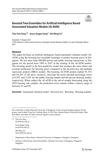
T. Sing et al.Fig. 2 The in-house designed Boosting Model. Note: The figure shows the flow chart of the boostingensemble method, which sequentially identifies the “weak learners” and corrects the errors to change theweak learners into strong learnersThe right-hand panel of Fig. 2 uses an inverted tree representation for the decision tree, where the splitting starts from the root at the top and moves downward sequentially. The first split is at the region [X1 t1] into two branches, oneis defined by [ X1 t1] and another by [ X1 t1]; and then the left-hand branch, [X1 t1], is further split at the region, [ X2 t2]. For the right-hand branch, [X1 t1], the split occurs at [ X1 t3]; and then the branch, [ X1 t3] is further splitat [X2 t4]. The splitting process continues till some stopping rules are applied.For a response, (xi, yi), such that [i 1, 2, .p], where p denotes the numberof observations (inputs), the split variables and the split points are automatically decided by the algorithm that defines a tree topology. The feature space isdivided into M regions by several rules (constants), [R1, R2, ., RM], which canbe defined as follows:f (x) M m 1()cm I x Rm(1)The decision tree mimics closely the way a human makes decisions, which aresometimes represented by qualitative predictors. Decision trees use a simple tointerpret graphical representation, but the prediction of a decision tree is not asstable as the regression models. A small change in data could cause a big changein outcomes. To overcome the limitations, two ensemble methods that are bagging and boosting are used in this study to aggregate multiple decision trees.However, a large ensemble of decision trees could potentially increase computational time, especially when the dataset used is also large.13
Boosted Tree Ensembles for Artificial Intelligence Based Tree Ensemble Methods: Bagging and BoostingOne major limitation of the decision tree method is the high variance in outcomes.When we divide the data into a training dataset and a testing dataset, we may obtaindifferent results every time when we fit a decision tree to different datasets. Thereare various ensemble approaches used to reduce variances in the outcomes. Thisstudy uses bagging and boosting methods, where the boosting is a relatively moreefficient method in term of computational time (see the next section for details).Bagging uses the bootstrap method to first generate B sets of different bootstrapped training data repetitively from a single training data set. After building aseparate decision tree from the B training data sets, the next step in the bagging process is to average the sets of observations to reduce variances, and in turn increaseaccuracy in prediction.In bagging, each tree is built on a bootstrapping data set that is independent ofother trees. However, in boosting method, the trees are grown sequentially from theprevious trees. The trees constructed by the boosting method is strongly dependenton the earlier trees that have been grown.2 The output of the boosting model can beformulated as below: f (x) B 𝜆f b (x)(2)b 1where b is the number of repetitive times from 1 to B, and λ is the shrinkageparameter with a typical value set at between 0.01 and 0.001.Estimating ProceduresBased on the proposed tree-based model, we compute the original residual, which isdefined as the difference between the actual housing value (dependent variable) andthe predicted housing value. The “weak learners”, which are assigned more weightsbased on the residual errors. The boosting method repeatedly and sequentially corrects and fits the residuals of “weak learners” by the predecessors in a bootstrappingprocess. The boosting method reduces variance and bias in the tree ensemble byconverting “weak learners” into “strong learners” in the process.We start by building a small decision tree with just a few terminal nodes. Weexpand and add new trees to the ensemble of trees that have already been grown. Weimprove the performance of the small tree steps by steps by reducing the shrinkageparameters.Three parameters are used to measure the efficacy and the speed of the learning process. The first parameter is the number of trees B, where a large B indicatespositive performance of the decision trees. However, the optimal B must be carefullyselected through a cross-validation process to avoid overfitting of the model, which2The trees in the boosting method are path dependence by nature (Ruppert, 2004), and this is an important feature widely observed in real estate appraisals. More discussions are included in the next section.13
T. Sing et al.occurs by having a very large B. The second parameter is the shrinkage parameter, λ,which controls the rate of the boosting in the learning process; and this number typically falls within a small range between 0.01 and 0.001. A good model should have avery small λ and a large B. The third parameter d is the number of splits in each treethat defines the interaction order of the boosting model. A model with a large d has amore complex boosted tree structure with the required depth in interactions.In the boosting model, a loss function is selected as the optimization target bya stepwise optimizing algorithms for a typical regression tree, which are definedbelow:1. Set f̂ (x) 0andri yi for all i in the training set.2. For b 1, 2, , B, repeat:a. Fit a tree f̂ b with d splits (d 1 terminal nodes) to the training data (X, r).b. Update f̂ by adding in a shrunken version of the new tree:f̂ (x) f̂ (x) 𝜆f̂ b (x).c. Update the residuals,( )ri ri 𝜆f̂ b xi .Output the Boosted Modelf̂ (x) B 𝜆f̂ b (x).b 1Figure 2 shows the flowchart of the Boosting algorithms, which can be broadlydivided into the following steps:1. To train a weak classifier using the training dataset;2. To adjust training dataset to allow conversion of the weak classifier using a predefined strategy;3. To repeat the training of other weak classifiers using the same approach (can bedone in parallel distributed computational process). All weak classifiers in theboosting can be different;4. To combine the weak classifiers obtained from the previous training to form astrong classifier; and5. To improve the accuracy of a given learning algorithm.Predictive Performance MeasuresA “horserace” can be conducted for the tree-based AI-AVM models that account fornon-linearity in the predictive relationships against the traditional multiple regression (MRA) models. We assess the predictive performance of the proposed AI-AVM13
Boosted Tree Ensembles for Artificial Intelligence Based and MRA models using three performance measures, which include R2, Root meansquare error (RMSE) and Mean absolute percentage error (MAPE).Let yiand ŷi represent the actual housing price and the predicted price, respectively. The absolute error is defined:ei yi ŷi (3)The R-square, ( R2), which is also known as coefficient of determination, with avalue bounded between 0 and 1 is defined in percentage term as: 2 N yi ŷii 12R 1 (4) 2Ny yiii 1where yi is the mean housing price, and N is the number of cases.The root means square error, (RMSE) is defined as: N 1 ()2 RMSE y ŷiN i 1 iThe scaled mean absolute percentage error (MAPE) is defined as:)(N100% yi ŷi MAPE yi Ni 1 (5)(6)R2 measures variance in a dependent variable that is accounted for by predictorsin the model; and a better performed model should have a higher R 2 value. However,a smaller value for RMSE and MAPE implies more accurate predictions.By randomly splitting the data into a training dataset and a test dataset, we repeatthe estimations by 50 times for each training-test split set to enable the convergencein the prediction accuracy. We derive the three indices for each of the random iteration and then calculate the average R2, RMSE and MAPE as the model’s predictionperformance measures.Applications of the Proposed AI‑AVMThis sections illustrates how the proposed AI-AVM developed using the decisiontree and boosting technique is applied to appraise private and public housing valuesin Singapore.Housing Markets in SingaporeSingapore has one of the highest home ownership rates in the world. Every ninein 10 public housing dwellers own their flats in Singapore as of 2020. The HomeOwnership Scheme introduced in 1964 has been one of the key pillars underpinning13
T. Sing et al.Singapore’s public housing system, which is enviable to many countries facing acutehousing shortage problems.Singapore housing market is characterized by a two-tier housing market comprising a public market and a private market. The public housing market forms a rocksolid base where nearly 1.08 million public housing flats currently serves the housing needs of more than 78% of Singapore residents. Public housing flats providenew starter houses at subsidized rates for first time home buyers, who meet specifiedsocial, demographic and income criteria.3 There is a formal resale market for publichousing units, where prices are market determined. The public housing wealth canonly be cashed out by the households upon satisfying a 5-year minimum occupancyrequirement. The difference in price between the new and resale public housing markets creates housing wealth to the first-time home buyers. The financial gains fromselling the starter houses provide an important source of funding for down paymentsfor liquidity constrained households in trading-up for private (trade-up) houses.The private housing market in Singapore operates on a laissez faire basis. Privatehousing units are more expensive. They are also differentiated by better designs,quality of finishes, and some (condominiums and apartments) are equipped withfull recreational facilities. Despite the relatively small scale of the private housingmarket, housing types are more heterogeneous and range from landed units likedetached houses, semi-detached houses and terraces to non-landed units like condominiums and apartments.Input Data and VariablesThe preliminary steps in estimating the AI-AVM model involve data collection, cleaning and coding of input variables. We collect a big dataset consisting of378,032 transactions from both the private and the public (resale) housing marketsin Singapore covering the period from 1995 to 2019. We drop observations withincomplete and missing data, and truncate 1% of the samples at both tails of the distributions to eliminate outliers. We then split the dataset into a training dataset anda testing dataset by a ratio of 9:1. The data analyses are conducted using the algorithms written in the R program.In addition to the transaction unit price, which is the dependent variable of themodel, the data include a list of hedonic property and spatial attributes, such as unitsize, floor level, tenure, sale type, project name and sale date, which are used as thepredictors in the proposed AI-AVM model. Table 1 describes the list of variables.Adjusting for Lagged Price EffectsAppraisers use past transactions as comparable in the price adjustment process. When the appraised values are closely anchored to the past reference point,3See Phang (2004) and Sing et al. (2006) for detailed discussions of policy changes affecting the publichousing market in Singapore over time.13
Boosted Tree Ensembles for Artificial Intelligence Based Table 1 Description of variablesVariableDescription(A) For private housing modelUpricetransacted unit price (S per square meter);FloorFloor level (height) of property (storey);AreaUnit size (square meters, sm);MonthThe month in the transaction date, [1, 2, 12];YearThe year of the transaction, [1995 to 2019];FreeholdLand tenure that has a value of 1, if it is a freehold land and a leaseholdland of more than 900 years; and otherwise 0; (only for private housing)Dist cityDistance to the CBD (km);Dist MRTDistance to the nearest MRT station (in km);PypThe average transaction unit price of the same project in the previousone year (S per square meter)(B) For Public Housing modelUpricetransacted unit price (S per square meter);FloorFloor level (height) of property (in storey);AreaUnit size (square meters, sm);MonthThe month in the transaction date, [1, 2, 12];YearThe year of the transaction, [1995 to 2019];Dist cityDistance to the CBD (km);Dist MRTDistance to the nearest MRT station (in km);PypThe average transaction unit price of the same project in the previousone year (S per square meter)Note: The table summarizes a list of variables with the descriptions that are used in constructing thehousing price models using the decision-tree, boosting and multivariate regression analysis (MRA)methods. The top panel includes the variables from the private housing market, and the bottom panelincludes variables from the public housing market. The freehold dummy variable is only found in the toppanel, which has a value of 1, if a land has freehold tenure or leasehold tenure of more than 900 years;and 0 otherwise. The dummy is not used in the public housing market, which has the same 99-year leasehold tenureappraised values could be out-of-sync with market prices in both up and down-markets (Fisher et al., 1999). The price index constructed from appraised values of afixed portfolio of real estate tend to understate the true market volatility and exhibitstrong lagged-relationships; and the problem is commonly known as “appraisalsmoothing” in the literature (Geltner, 1989). Geltner (1989, 1991), Quan and Quigley (1991) and other researchers have proposed ways to “unsmooth” (de-lag) theappraisal-based indices to uncover the “true” real estate return. The approach addsserial-correlations (lagged auto-regressive term) back to the appraisal-based returnsto infer the true returns.In an inefficient housing market, serial correlations could also exist in prices becauseof the slow price discovery process. Case and Shiller (1980 and Case & Shiller, 1990)found evidence of correlated real price changes in the short-term using repeated13
T. Sing et al.Table 2 Descriptive StatisticsvariablemeanminmaxSDUnit Price (S psm)uprice3288.711963.415462.69927.33Floor level (storey)floor7.52384.41Unit area (sqm)area96.933128025.25Building age (year)age29.495529.33Year of saleyear2007.97200120174.57Month of Salemonth6.461123.4Distance to the nearest MRT station (km)dist MRT0.70.012.810.46Distance to CBD (km)dist city11.61.418.43.86Previous year unit (S psm) pricePyp3168.51963.775462.69866.05Unit Price (S psm)uprice9655.643965.5227,133.333720.12Floor level (storey)floor8.361666.78Unit area (sqm)area126.2224121253.26Building age (year)age10.731647.29Freehold tenure dummyfreehold0.49010.5Year of saleyear2009.56199620195.65Month of Salemonth6.221123.18Distance to the nearest MRT station (km)dist MRT1.090.035.750.78Distance to CBD (km)dist city7.30.424.43.9Previous year unit (S psm) pricePyp9051.133965.5219,658.113601.59(A) Public Housing Market(B) Private Housing MarketNote: The table provides the summary statistics, which include the mean, minimum, maximum andstandard deviation (SD) for the list of the outcome variables and predictors. The top panel (A) shows theresults for the private housing market, and the bottom panel (B) shows the results for the public housingmarkettransactions in the single-family housing markets in the selected US cities. The twostrands of literature are not mutually exclusive; it is difficult to disentangle serial correlations (appraisal smoothing) in the transaction prices and appraised values. However, it isnot the intent of our study to separate serial correlations in our model; instead, recognizing the inefficiency in the housing markets, our AI-AVM models incorporate the laggedprice variable, which is the average transaction prices at the project level in the previousyear, to improve the predictability of housing prices.4Descriptive StatisticsTable 2 shows the descriptive statistics of mean, minimum, maximum, and standard deviation of both the dependent vari
study develops the AI automated valuation models (AI-AVM) for residential properties using the established approaches, such as decision tree and/or boosting methodologies. There are two unique features of our proposed AI-AVM: First, we use the bagging and boosting method to capture inter-dependency in the deci-sion tree in the ANN model.