Transcription
Schonlau M. Boosted Regression (Boosting): An introductory tutorial and a Stataplugin. The Stata Journal, 5(3), 330-354.Boosted Regression (Boosting): An introductory tutorial and a StatapluginMatthias SchonlauRANDAbstractBoosting, or boosted regression, is a recent data mining technique that has shownconsiderable success in predictive accuracy. This article gives an overview over boostingand introduces a new Stata command, boost, that implements the boosting algorithmdescribed in Hastie et al. (2001, p. 322). The plugin is illustrated with a Gaussian and alogistic regression example. In the Gaussian regression example the R2 value computedon a test data set is R2 21.3% for linear regression and R2 93.8% for boosting. In thelogistic regression example stepwise logistic regression correctly classifies 54.1% of theobservations in a test data set versus 76.0% for boosted logistic regression. Currently,boost accommodates Gaussian (normal), logistic, and Poisson boosted regression. boostis implemented as a Windows C plugin.1
1 IntroductionEconomists and analysts in the data mining community differ in their approach toregression analysis. Economists often build a model from theory and then use the data toestimate parameters of their model. Because their model is justified by theory economistsare sometimes less inclined to test how well the model fits the data. Data miners tend tofavor the “kitchen sink” approach in which all or most available regressors are used in theregression model. Because the choice of x-variables is not supported by theory, validationof the regression model is very important. The standard approach to validating models indata mining is to split the data into a training and a test data set.The concept of training versus test data set is central to many data miningalgorithms. The model is fit on the training data. The fitted model is then used to makepredictions on the test data. Assessing the model on a test data rather on the training dataensures that the model is not overfit and is generalizable. If the regression model hastuning parameters (e.g. ridge regression, neural networks, boosting), good values for thetuning parameters are usually found running by the model several times with differentvalues for the tuning parameters. The performance of each model is assessed on the testdata set and the best model (according to some criterion) is chosen.In this paper I review boosting or boosted regression and supply a Stata plugin forWindows. In the same way that generalized linear models include Gaussian, logistic andother regressions, boosting also includes boosted versions of Gaussian, logistic and otherregressions. Boosting is a highly flexible regression method. It allows the researcher tospecify the x-variables without specifying the functional relationship to the response.Traditionally, data miners have used boosting in the context of the “kitchen sink”approach to regression but it is also possible to use boosting in a more targeted manner,i.e. using only variables motivated by theory. Because it is more flexible, a boostedmodel will tend to fit better than a linear model and therefore inferences made based onthe model may have more credibility.There is mounting empirical evidence that boosting is one of the best modelingapproaches ever developed. Bauer and Kohavi (1999) performed an extensivecomparison of boosting to several other competitors on 14 datasets, and found boosting to2
be “the best algorithm”. Friedman et al. (2000) compare several boosting variants to theCART (classification and regression tree) method and find that all the boosting variantsoutperform the CART algorithm on eight datasets.The success of boosting in terms of predictive accuracy has been subject to muchspeculation. Part of the mystery that surrounds boosting is due to the fact that differentscientific communities, computer scientists and statisticians, have contributed to itsdevelopment. I will first give a glimpse into the fascinating history of boosting.The remainder of the paper is structured as follows: Section 2 contains the syntaxof the boost command. Section 3 contains options for that command. Section 4 explainsboosting and gives a historical overview. Section 5 uses a toy example to show how theboost command can be used for normal (Gaussian) regression. Section 6 features alogistic regression example. Section 7 gives runtime benchmarks for the boostingcommand. Section 8 concludes with some discussion.2 Installation and SyntaxTo install the boost plugin copy the boost.hlp and boost.ado files in one of the adodirectories, e.g. c:\ado\personal\boost.ado . A list of valid directories can be obtained bytyping “adopath” within Stata. Copy the “boost.dll” file into a directory of your choosing(e.g. the same directory as the ado file). Unlike an ado file, a plugin has to be explicitlyloaded:capture program boost plugin, plugin using("C:\ado\personal\boost.dll")The command "capture" prevents this line resulting into an error in case the plugin wasalready loaded. The command syntax is as follows:boost varlist [if exp] [in range] , DISTribution(string) maxiter(int)[ INfluence PREDict(varname) shrink(real 0.01)bag(real 0.5) INTERaction(int 5) seed(int 0) ]3
3 Optionsboost determines the number of iterations that maximizes the likelihood, or, equivalently,the pseudo R squared. The pseudo R2 is defined as R2 1-L1/L0 where L1 and L0 are thelog likelihood of the full model and intercept-only model respectively.Unlike the R2 given in regress, the pseudo R2 is an out-of-sample statistic. Out-ofsample R2's tend to be lower than in-sample-R2's.Output and Return valuesThe standard output consists of the best number of iterations, bestiter, the R squaredvalue computed on the test data set, test R2, and the number of observations used forthe training data, trainn. trainn is computed as the number of observations that meet thein/if conditions times trainfraction. These statistics can also be retrieved using ereturn.In addition, ereturn also stores the training R squared value, train R2, as well as the loglikelihood values from which train R2 and test R2 are computed.distribution(string) Currently, possible distributions are "normal", "logistic", and"poisson".influence displays the percentage of variation explained (for non-normal distributions:percentage of log likelihood explained) by each input variable. The influence matrix issaved in e(influence).predict(varname) predicts and saves the predictions in the variable varname. To allow forout-of-sample predictions predict ignores if and in. For model fitting only observationsthat satisfy if and in are used, predictions are made for all observations.trainfraction(int) Specifies the percentage of data to be used as training data. Theremainder, the test data is used to evaluate the best number of iterations. By default thisvalue is 0.8.interaction(int) specifies the maximum number of interactions allowed. interaction 1means that only main effects are fit, interaction 2 means that main effect and two wayinteractions are fitted, and so forth. The number of interactions equals the number ofterminal nodes in a tree plus 1. If interaction 1, then each tree has 2 terminal nodes. If4
interaction 2, then each tree has 3 terminal nodes, and so forth. By defaultinteraction 5.maxiter(int) specifies the maximal number of trees to be fitted. The actual number used,bestiter, can be obtained from the output as e(bestiter). When bestiter is too close tomaxiter the maximum likelihood iteration may be larger than maxiter. In that case it isuseful to rerun the model with a larger value for maxiter. When trainfraction 1.0 allmaxiter observations are used for prediction (bestiter is missing because it is computedon a test data set).shrink(#) specifies the shrinkage factor. shrink 1 corresponds to no shrinkage. As ageneral rule of thumb, reducing the value for shrink requires an increase in the value ofmaxiter to achieve a comparable cross validation R2. By default shrink 0.01.bag(real) Specifies the fraction of training observations that is used to fit an individualtree. bag 0.5 means that half the observations are used for building each tree. To use allobservations specify bag 1.0.By default bag 0.5.seed(int) seed specifies the random number seed to generate the same sequence ofrandom numbers. Random numbers are only used for bagging. Bagging uses randomnumbers to select a random subset of the observations for each iteration. By default(seed 0). The boost seed option is unrelated to Stata's set seed command.4 BoostingBoosting was invented by computational learning theorists and later reinterpretedand generalized by statisticians and machine learning researchers. Computer scientiststend to think of boosting as an “ensemble” method (a weighted average of predictions ofindividual classifiers), whereas statisticians tend to think of boosting as a sequentialregression method. To understand why statisticians and computer scientists think aboutthe essentially same algorithms in different ways, both approaches are discussed. Section4.1 discusses an early boosting algorithm from computer science. Section 4.2 describesregression trees, the most commonly used base learner in boosting. Section 4.3 describesFriedman’s gradient boosting algorithm, which is the algorithm I have implemented for5
the Stata plugin. The remaining sections talk about variations of the algorithm that arerelevant to my implementation (Section 4.4), how to evaluate boosting algorithms via across validated R2 (Section 4.5), the influence of variables (Section 4.6) and advice onhow to set the boosting parameters in practice (Section 4.7).4.1 Boosting and its roots in computer scienceBoosting was invented by two computer scientists at AT&T Labs (Freund andSchapire, 1997). Below I describe an early algorithm, the “AdaBoost” algorithm,because it illustrates why computer scientists think of boosting as an ensemble method;that is, a method that averages over multiple classifiers.Adaboost (see Algorithm 1) works only in the case where the response variabletakes only one of two values: -1 and 1. (Whether the values are 0/1 or –1/1 is notimportant- the algorithm could be modified easily). Let C1 be a binary classifier (e.g.logistic regression) that predicts whether an observation belongs to the class “-1” or “1”.The classifier is fit to the data as usual and the misclassification rate is computed. Thisfirst classifier C1 receives a classifier weight that is a monotone function of the error rateit attains. In addition to classifier weights there are also observation weights. For thefirst classifier, all observations were weighted equally. The second classifier, C2 (e.g.the second logistic regression), is fit to the same data, however with changed observationweights. Observation weights corresponding to observations misclassified by theprevious classifier are increased. Again, observations are reweighted, a third classifier C3(e.g. a third logistic regression) is fit and so forth. Altogether iter classifiers are fit whereiter is some predetermined constant. Finally, using the classifier weights theclassifications of the individual classifiers are combined by taking a weighted majorityvote. The algorithm is described in more detail in Algorithm 1.6
Initialize weights to be equal wi 1/nFor m 1 to iter classifiers Cm):(a)Fit classifier Cm to the weighted data(b)Compute the (weighted) misclassification rate rm(c)Let the classifier weight αm log ( (1 – rm)/rm )(d)Recalculate weights wi wi exp(αm I(yi Cm )) M Majority vote classification: sign α m C m (x ) m 1 Algorithm 1: The AdaBoost algorithm for classification into two categories.Early on, researchers attributed the success and innovative element of thisalgorithm to the fact that observations that are repeatedly misclassified are givensuccessively larger weights. Another unusual element is that the final “boosted”classifier consists of a majority-weighted vote of all previous classifiers. With thisalgorithm, the individual classifiers do not need to be particularly complex. On thecontrary, simple classifiers tend to work best.4.2 Regression treesThe most commonly used simple classifier is a regression tree (e.g. CART,Breiman et al.,1984). A regression tree partitions the space of input variables intorectangles and then fits a constant (e.g. estimated by an average or a percentage) to eachrectangle. The partitions can be described by a series of if-then statements or they can bevisualized by a graph that looks like a tree. Figure 1 gives an example of such a tree usingage and indicator variables for race/ethnicity. The tree has 6 splits and therefore 7 leaves(terminal nodes). Each split represents an if-then condition. Each observation descendsthe set of if-then conditions until a leaf is reached. If the if-then condition is true then theobservation goes to the right branch otherwise to the left branch. For example, in Figure 2any observation over 61 years of age would be classified in the right most leaf regardless7
of his/her race/ethnicity. The leaf with the largest values of the response, 0.8, correspondsto observations between 49 and 57 years of age, who are neither Hispanic nor Black. Asthe splits on age show, the tree can split on the same variable several times. If the 6 splitsin the tree in Figure 1 had split on six different variables the tree would represent a 6level interaction because six variables would have to be considered jointly in order toobtain the predicted value. age 61age 130.73asian 0.50.20age 570.21hispan 0.50.29age 490.330.520.80Figure 1: Example of a regression tree with 6 splitsA regression tree with only two terminal nodes (i.e., a tree with only one split) iscalled a tree stump. It is hard to imagine a simpler classifier than a tree stump – yet treestumps work surprisingly well in boosting. Boosting with stumps fits an additive modeland many datasets are well approximated with only additive effects. Fewer, complexclassifiers can be more flexible and harbor a greater danger of overfitting (i.e., fitting wellonly to the training data).8
4.3 Friedman’s gradient boosting algorithmEarly researchers had some difficulty explaining the success of the AdaBoostalgorithm. The computational learning theory roots of the AdaBoost puzzled statisticianswho have traditionally worked from likelihood-based approaches to classification and,more generally, to regression. Then Friedman et al. (2000) were able to reinterpret thisalgorithm in a likelihood framework, enabling the authors to form a boosted logisticregression algorithm, a formulation more familiar to the statistical community. Once theconnection to the likelihood existed, boosting could be extended to generalized linearmodels and further still to practically any loss criterion (Friedman 2001, Ridgeway,1999). This meant that a boosting algorithm could be developed for all the errordistributions in common practice: Gaussian, logistic, Poisson, Cox models, etc. With thepublication of Hastie et al. (2001), a book on statistical learning, modern regressionmethods like boosting caught on in the statistics community.The interpretation of boosting in terms of regression for a continuous, normallydistributed response variable is as follows: The average y-value is used as a first guess forpredicting all observations. This is analogous to fitting a linear regression model thatconsists of the intercept only. The residuals from the model are computed. A regressiontree is fit to the residuals. For each terminal node, the average y-value of the residualsthat the node contains is computed. The regression tree is used to predict the residuals.(In the first step, this means that a regression tree is fit to the difference between theobservation and the average y-value. The tree then predicts those differences.) Theboosting regression model - consisting of the sum of all previous regression trees - isupdated to reflect the current regression tree. The residuals are updated to reflect thechanges in the boosting regression model; a tree is fit to the new residuals, and so forth.This algorithm is summarized in more detail in Algorithm 2.1) Initialization: Set initial guess to y2) For all regressions trees m 1 to M:2a) Compute the residuals based on the current model9
rmi yi – fm-1(xi)where i indexes observations.Note that fm-1 refers to the sum of all previous regression trees.2b) Fit a regression tree (with a fixed number of nodes) to the residuals2c) For each terminal node of the tree, compute the average residual. The averagevalue is the estimate for residuals that fall in the corresponding node.2d) Add the regression tree of the residuals to the current best fitfm fm-1 last regression tree of residualsAlgorithm 2: Friedman’s gradient boosting algorithm for a normally distributedresponseEach term of the regression model thus consists of a tree. Each tree fits theresiduals of the prediction of all previous trees combined. To generalize Algorithm 2 to amore general version with arbitrary distributions requires that “average y-value” bereplaced with a function of y-values that is dictated by the specific distribution and thatthe residual (Step 2a) be a “deviance residual”. (McCullagh and Nelder, 1989)The basic boosting algorithm requires the specification of two parameters. One isthe number of splits (or the number of nodes) that are used for fitting each regression treein step 2b of Algorithm 2. The number of nodes equals the number of splits plus one.Specifying one split (tree stumps) corresponds to an additive model with only maineffects. Specifying two splits corresponds to a model with main effects and two-wayinteractions. Generally, specifying J splits corresponds to a model with up to J-wayinteractions. When J x-variables need to be considered jointly for a component of aregression model this is a J-way interaction. Hastie et al. (2001) suggest that J 2 ingeneral is not sufficient and that 4 J 8 generally works well. They further suggestthat the model is typically not sensitive to the exact choice of J within that range. In theStata implementation J is specified as an option: interaction(J).10
The second parameter is the number of iterations or the number of trees to be fit.If the number of iterations is too large the model will overfit; i.e., it will fit the trainingdata well but not generalize to other observations from the same population. If thenumber of iterations is too small then the model is not fit as well either. A suitable valuefor maxiter can range from a few dozen to several thousand, depending on the value of ashrinkage parameter (explained below) and the data set. The easiest way to find asuitable number of iterations is to check how well the model fits on a test data set. In theStata implementation the maximal number of iterations, maxiter, is specified and thenumber of iteration that maximizes the log likelihood on a test data set, bestiter, isautomatically found. The size of the test data set is controlled by trainfraction. Forexample, if trainfraction 0.5 then the last 50% of the data are used as test data.4.4 Shrinkage and baggingThere are two commonly used variations on Friedman’s boosting algorithm:“shrinkage” and “bagging”. Shrinkage (or regularization) means reducing or shrinkingthe impact of each additional tree in an effort to avoid overfitting. The intuition behindthis idea is that it is better to improve a model by taking many small steps than a smallernumber of large steps. If one step turns out to be a misstep, then the damage can be moreeasily undone in subsequent steps. Shrinkage has been previously employed, forexample, in ridge regression where it refers to shrinking regression coefficients back tozero to reduce the impact of unstable regression coefficients on the model. Shrinkage isaccomplished by introducing a parameter λ in step 2d of Algorithm 2:fm fm-1 λ * (last regression tree of residuals)where 0 λ 1. The smaller λ, the greater the shrinkage. The value λ 1 corresponds tono shrinkage. Typically λ is 0.1 or smaller with λ 0.01 or λ 0.001 being common.Smaller shrinkage values require larger number of iterations. In my experience, λ and thenumber of iterations typically satisfy 10 λ * bestiter 100 for the best model. In otherwords, a decrease of λ by a factor of 10 implies an increase of the number of iterations bya similar factor. In the Stata implementation λ is specified through the option shrink(λ).The second commonly used variation on the boosting algorithm is bagging. Ateach iteration only a random fraction, bag, of the residuals is selected. In that iteration,11
only the random subset of the residuals is used to build the tree. Non-selected residualsare not used in that iteration at all. The randomization is thought to reduce the variationof the final prediction without affecting bias. Different random subsets may havedifferent idiosyncrasies that will average out. While not all observations are used in eachiteration, all observations are eventually used across all iterations. Friedman (2002)recommends the bagging with 50% of the data. In the Stata implementation this can bespecified as bag(0.5).4.5 Crossvalidation and the pseudo R2Highly flexible models are prone to overfitting. While it may still occur,overfitting is less of an issue in linear regression where the restriction of linearity guardsagainst this problem to some extent. To assess predictive accuracy with highly flexiblemodels it is important to separate the data the model was trained on from test data.My boosting implementation splits the data into a training and a test data set. Bydefault the first 80% of the data are used as training data and the remainder as test data.This percentage can be changed through the use of the option trainfraction. Iftrainfraction 0.5, for example, then the first 50% of the data are used as training data. Itis important that the observations are in random order before invoking the boostcommand because otherwise the test data may be different form the training data in asystematic way.Crossvalidation is a generalization of the idea of splitting the data into trainingand test data sets. For example, in five-fold crossvalidation the data set is split into 5distinct subsets of 20% of the data. In turn each subset is used as test data and theremainder as training data. This is illustrated graphically in Figure 2. Myimplementation corresponds to the fifth row of Figure 2. An example of how to rotatethe 5 groups of data to accomplish five-fold crossvalidation using the boostimplementation is given in the help file for the boost command.1test2train3traintesttraintraintesttrain12
4testtrain5traintraintestFigure 2: Illustration of five-fold cross validation: Data are split into training and testdata in five different ways.For each test data set a pseudo R2 is computed on the test data set. The pseudo R2is defined aspseudo R2 1- L1/L0where L1 and L0 are the log likelihoods of the model under consideration and anintercept-only model, respectively (see Long and Freese, 2003, for a discussion onpseudo R2). In the case of Gaussian (normal) regression, the pseudo R2 turns into thefamiliar R2 that can be interpreted as “fraction of variance explained by the model”. ForGaussian regression it is sometimes convenient to compute R2 asR2 Var ( y ) MSE ( y, yˆ )Var ( y )(1)where Var(.) and MSE(.,.) refer to variance and mean squared error respectively. Toavoid cumbersome language this is referred to as “test R2” in the remainder of this paper.The training R2 and test R2 are computed on training and test data, respectively.The training R2 is always between 0 and 1. Usually, the test R2 is also between 0 and 1.However, if the log likelihood based on the intercept-only model is greater than the onefor the model under consideration the test R2 is negative. A negative test R2 is a sign thatthe model is strongly overfit. The boost command computes both training and test R2values and makes them available in e(test R2) and e(train R2).4.6 Influence of variables and visualizationFor a linear regression model the effect of x-variables on the response variable issummarized by their respective coefficients. The boosting model is complex but can beinterpreted with the right tools. Instead of regression coefficients, boosting has theconcept of “influence of variables” (Friedman, 2001). Each split on a variable in aregression tree increases the log likelihood of the regression tree model. In Gaussianregression the increase in log likelihood is proportional to the increase in sums of squares13
explained by the model. The sum of log likelihood increases across all trees due to agiven variable yields the influence of that variable. For example, suppose there are 1000iterations or regression trees. Suppose that each regression tree has one split (i.e. a treestump, meaning interaction 1, meaning main effects only). Further, suppose that 300 ofthe regression trees split on variable xi. Then the sum of the increase in log likelihood dueto these 300 trees represents the influence of xi. The influences are standardized such thatthey add up to 100%.Because a regression tree does not separate main effects and interactions,influences are only defined for variables - not for individual main effect or interactionterms. Influences only reveal the sum of squares explained by the variables; they saynothing about how the variable affects the response. The functional form of a variable isusually explored through visualization. Visualization of any one (or a any set of)variables is achieved by predicting over a range or grid of these variables. Suppose theeffect of xi on the response is of interest. There are several options. The easiest is topredict the response for a suitable range of xi values while holding all other variablesconstant (for example at their mean or their mode). A second option is to predict theresponse for a suitable range of xi values for each observation in the sample. Then thesample-averaged prediction for a give xi value can be computed. A third option is tonumerically integrate out other variables with a suitable grid of values to get what isusually referred to as a main effect.In linear regression the coefficient of a variable need to be interpreted in thecontext of its range. It is possible to artificially inflate coefficients by, for example,changing a measurement from kilogram to gram. The influence percentages are invariantto any one-to-one rescaling of the variables. For example, measuring a variable in milesor kilometers does not affect the influence but it would affect the regression coefficient ofa logistic regression. In the Stata implementation the influence of individual variables isdisplayed when option influence is specified. The individual values are stored in a Statamatrix and can be accessed through e(influence). The help file gives an example.4.7 Advice on setting boosting parameters14
In what follows I give some suggestions of how the user might think about settingparameter values.Maxiter: If e(bestiter) is almost as large as maxiter consider rerunning the model with alarger value for maxiter. The iteration corresponding to the maximum likelihood estimatemay be greater than maxiter.Interactions: Usually a value between 3 and 7 works well. If you know your model onlyhas two-way interactions I still suggest trying larger values also for two reasons. One,typically, the loss in test R2 for specifying too low a number of interactions is far worsethan the one of specifying a larger number of interactions. The performance of the modelonly deteriorates noticeably when the number of interactions is much too large. Two,specifying 5-way interactions allows each tree to have 5 splits. These splits are notnecessarily always used for an interaction (splitting on 5 different variables in the sametree). They could also be used for a nonlinearity in a single variable (5 splits on differentvalues for a single variable) or for combinations of nonlinearities and interactions.Shrinkage: Lower shrinkage values usually improve the test R2 but they increase therunning time dramatically. Shrinkage can be thought of as a step size. The smaller thestep size, the more iterations and computing time are needed. In practice I choose a smallshrinkage value such that the command execution does not take too much time. Because Iam impatient, I usually start out with shrink 0.1. If time permits switch to 0.01 or lowerin a final run. There are diminishing returns for very low shrinkage values.Bagging: Bagging may improve the R2 and it also makes the estimate less variable.Typically, the exact value is not crucial. I typically use a value in the range of 0.4-0.8.5 Example: Boosted Gaussian regressionThis section gives a simple example with four explanatory variables constructedto illustrate how to perform and evaluate boosted regressions. The results are also15
compared to linear regression. Linear regression is a good reference model because manyscientists initially fit a linear model. I simulated data from the following modely 30( x1 0.5) 2 2 x2 0.5 x3 εwhere ε uniform(0,1) and 0 xi 1 for i 1, 2,3 . To keep things relatively simple, themodel has been chosen to be additive without interactions. It is quadratic in x1, nonlinearin x2, linear with a small slope in x3. The nonlinear contribution of x2 is stronger than thelinear contribution of x3 even though their slopes are similar. A fourth variable, x4, isunrelated to the response but is used in the analysis in an attempt to confuse the boosting002020y40y4060608080algorithm. Scatter plots of y vs x1 through x4 is shown in Figure 10.2.4.6.810x3.2.4x4Figure 3: Scatter plots of y versus x1 through x4I chose the following parameter values
Boosted Regression (Boosting): An introductory tutorial and a Stata plugin. The Stata Journal, 5(3), 330-354. Boosted Regression (Boosting): An introductory tutorial and a Stata plugin Matthias Schonlau RAND Abstract Boosting, or boosted regression, is a recent data mining technique that has shown considerable success in predictive accuracy.