Transcription
,\'"(" \I.,,'r .J. Water Resources Management10: 303-320, 1996.303@ 1996 Kluwer Academic Publishers. Printed in the Netherlands.;. .Estimation of Baseflow Recession ConstantsRICHARD M. VOGEL;)Departmentof Civil and A 02155,U.S.A.,e-mail: rvogel@tufts.edu.'c.,' ,andCHARLESN. KROLLResearch Associate, Department of Civil and Environmental Engineering, Cornell University,Ithaca, N. 14853, U.S.A.(Received: 17 February 1995; in final form: 30 August 1995)Abstract. Hydrograph recession constants are required in rainfall-runoff models, baseflow augmentation studies, geohydrologic investigations and in regional low-flow studies. The recession portionof a streamflow hydrograph is shown to be either an autoregressive process or an integrated movingaverage process, depending upon the structure of the assumed model errors. Six different estimatorsof the baseflow recession constant are derived and tested using thousands of hydrograph recessionsavailable at twenty-three sites in Massachusetts, U.S. When hydrograph recessions are treated as anautoregressive process, unconditional least squares or maximum likelihood estimators of the baseflow recession constant are shown to exhibit significant downward bias due to the short lengths ofhydrograph recessions. The precision of estimates of hydrograph recession constants is shown todepend heavily upon assumptions regarding the structure of the model errors. In general, regressionprocedures for estimating hydrograph recession parameters are generally preferred to the time-seriesalternatives. An evaluation of the physical significance of estimates of the baseflow recession constant is provided by comparing regional regression models which relate low-flow statistics to threeindependent variables: drainage area, basin slope and the baseflow recession constant. As anticipated,approximately unbiased estimators of the baseflow recession constant provide significant informationregarding the geohydrologic response of watersheds.Key words: baseflow recession constant, hydrograph, low flows, recession analysis. hydrogeology,streamflow.!1. Introduction',.,-,!, :,('.":Jj&:.i.:;"('101.' j",iTallaksen(1995) reviewsthe applicationof baseflowrecessionconstantsfor forecasting low flows, hydrograph analysis, low-flow frequency analysis, and fordescribingaquifer characteristics.Estimatesof hydrographrecessionconstantsarerequiredfor the calibration of rainfall-runoff modelsand in somecasesfor fittingstochasticstreamflowmodels(Kelman, aseflowrecessionconstantsareusedroutinelyfor modelingsurfacerunoff (Batesand Davies, 1988)and for constructingunit hydrographsby separating thebaseflowcomponentof streamflowfrom thetotal streamflowto obtaindirectrunoff. With increasingattentionfocusedon thequality andquantityof groundwater,understandingthecontributionof groundwaterto streamflow(baseflow)is often
,r,,,,. i;1 ",f ",304.:-."; '. 4. , :i ;;;; c' -"; z 1 ; d ];! ""c "-C'".h j };f;c'f:' -;::;:::}i 1 '.,' cc.,, ;: ':,,-,"'i' ".,:.: - .,.c'""C;"'?(C"',C:;I;- c:?r:;, -",;,c'. t'".c: '""':'cM. VOGELAND CHARLES N. KROLLIthe focus of applied groundwater studies. Ponce and Lindquist (1990) review man-.c"'.cRICHARDagement strategies for eight general types of baseflow augmentation applications,all of which require characterization of baseflow recessions.Riggs (1961), Bingham (1986), Vogel and Kroll (1992), Demuth and Hagemann (1994), this study, and others show that regional models which relate lowflow statistics to basin characteristics, can be significantly improved by using thebaseflow recession constant as one of the independent basin parameters.Vogel andKroll (1992) show that the baseflow recessionconstant is related to both the basinhydraulic conductivity and drainable soil porosity. Regional models for estimatinglow-flow statistics are used routinely at ungaged sites for the purposes of bothwater quality and water quantity management (see Vogel and Kroll, 1990, 1992,for discussions).Since the introduction of graphical hydrograph separation proceduresby Barnes(1939), a variety of approaches have been developed for separating baseflow fromthe total streamflow hydro graph. Barnes (1939) graphical hydro graph separationProcedures are still included in most introductory hydrolo gy textbooks in Spiteof the serious criticisms voiced by Kulandaiswamy and Seetharaman (1969) l(1971)and;Brutsaertand Nieber (1977) introduced alternative graphical procedures for hydrograph separation which contain fewer subjective judgements then the graphical procedures'.introduced by Barnes. A variety of analytic procedures have also been advancedtoprovide a more objectiveapproachto hydrographseparation(Jamesand Thomp-,:son (1970), Jones and McGilchrist (1978), Birtles (1978) and others). A review ofstudies relating to baseflow recession was performed by Hall (1968) and Tallaksen(1995).Recession constants must be estimated from an individual or an ensemble ofhydrographs; but in either case,derived estimatesare random variables whose physical significance should only be determined after an evaluation of their statisticalsignificance. To our knowledge, there are no studies which evaluate the statisticalproperties of estimated values of baseflow recession constants. One could perform bootstrap experiments with actual streamflow data, however still, one neverknows the true values of the baseflow recession constant, hence such experimentscannot be definitive. Alternatively, one could perform Monte-Carlo experiments,making certain assumptions regarding the true underlying structure of hydrographrecessions. Again, such experiments are not completely definitive because one.1never knows the true structure of hydro graph recessions. Thus, it is very difficultto discern whether any of the available graphical or analytical estimation procedures provide, for example, minimum variance and/or unbiased estimates of thetrue baseflow recession constant. Our approach is to focus on both the physicaland statistical significance of the resulting estimators. After presenting the theoryof hydrograph recessions and six plausible estimators of the baseflow recessionconstant, experiments are performed to evaluate the alternative estimators in termsof their ability to explain the geohydrologic or groundwater outflow response of;-' ";,,, ,. -.I
, , ;30523 watershedsin Massachusetts.Theseexperimentsareno more or lessdefinitive.!than Monte-Carlo or Bootstrap experiments would be, yet they do allow us todiscriminate among the alternate estimators.2. HydrographRecessionsBarnes (1939) found that hydro graph recessions seem to follow the basic relations c.;Bt I KbBt,(la)Ot I KoOt,(lb)where Bt and Ot are the baseflow and other (or remaining) component of streamflow, respectively, on day t and Kb and Ko are the baseflow and other recessionconstant, respectively. These two components of the recession streamflow sum toproduce the total streamflow, thusQt Bt at,(2)where Qt is the average daily streamflow on day t. Interestingly, Equation (la) isan approximate linear solution to the nonlinear differential equation which governsthe unsteady flow from a large unconfined aquifer to a stream channel (Boussinesq,1877; Singh, 1968; Singh and Stall, 1971; Brutsaert and Nieber, 1977; Vogel andKroll, 1992, etc.). Boussinesq (1904) obtained an equation similar to (2) using theprinciple of superposition of linear solutions. Brutsaert and Nieber (1977), Vogeland Kroll (1992) and others show how (1 a) or (1b) can be derived by treating thewatershed as a linear reservoir.Equations (1) and (2) .may be expressed in a variety of different forms (Hall,1968; Tallaksen, 1995), each of which leads to different estimation procedures.In the following sections we derive six different estimators of the baseflow recession constant, Kb, using the model described by (1) and (2). Using thousands ofstreamflow hydro graphs at 23 basins in Massachusetts,we compare both the physical and statistical properties of the four baseflow recession constant estimationprocedures.3. A Hydrograph Recessionis a Time SeriesIn the following sections, Equations (1) and (2) are rearranged to show that hydrograph recessions arise from an autoregressiveprocess.3.1. BASEFLOWRECESSIONAS AN AR(I)PROCESSEquations (1) and (2) describe a streamflow hydrograph without accounting for theinherent model error introduced by Boussinesq's linear approximation, measurement errors associated with all streamflow measurementsor sampling error arisingIL--
'"- -,,.:.306;from the fact that all streamflow records are of finite and often small duration. Due.IIRICHARD M. VOGEL AND CHARLES N. KROLLto these naturally occurring errors Equation (la) is more realistically KbBt E:t lBt l.(3)where the E:t are independent normally distributed errors with zero mean andconstant variance. The random errors are a result of both measurementand modelerrors. Equation (3) provides a reasonable approximation to the baseflow portionof a streamflow hydrograph recession because the other component(s) will havedecayed to zero. Equation (3) is a first-order autoregressive process, AR(I),the baseflow recession curve asan ARMA(I, 1) processwith Kb cPl (}l. Of course1970, the Box and Jenkins notation was unavailable. An ARMA(I,I)processwithJamesand Thompsondid not call their model an ARMA(I,I) processbecausein ','.',;,cPlIwhereKbis y BoxandJenkins(1976)for an AR(I)parameter.process,Kb cPl.Jamesand Thompsonderive-\.II'I[ (}l containsparameterredundancy(seeBox andJenkins,1976,pp. 248-250),thus the process reduces to white noise, making their analysis questionable.;;C:i':'3.2.BASEFLOW AS AN INTEGRATED MOVING AVERAGE PROCESSRewriting (3), assumingadditiveerrorsin log space,oneobtainsBt KbBt-leEt.(4)Experimentsperformedlater on indicatethat the error structureimposedin (4) ismore representativeof actual streamflowrecords.Equation (4) can be rewrittenusing Box and Jenkins(1976) notationby taking logarithmsand rearrangingtoIobtainYti- Yt-lwhere Yt In(Bt)f In(Kb)and Yt-l E:t In(Bt-l),\7Yt,(5)again the residuals are independent, withi[zero mean and constantvariance.Box and Jenkins(1976) term (5) an integrat-!ed moving average model IMA(O,I,O) with constant drift parameter In(Kb). Boxand Jenkins (1976) provide a discussion of the properties of nonstationary IMAmodels.3.3. THE HYDROGRAPHRECESSIONAS AN AR(2) PROCESSIf the baseflow and other component of a hydro graph are considered, then Equations (1) and (2) may be rewritten asQt I KbBt KoOt E:t l,(6)where the residuals E:tare independent and identically distributed random errorswith zero mean and constant variance. Using (la) and (lb), (6) may be rearrangedas follows:\ . ".Jt.j"", """"""
','r-;T.'.';.'",\':'-; i!! 1I,''.:E I, r.307ESTIMATION OF BASEFLOW RECESSIONCONSTANTSQt 1" Kb(Bt at) -KbOt Ko(Ot Bt)-KoBt E:t 1", (Kb Ko)(Bt at). (Kb- KbKoOt-1 - KoKbBt-1 E:t 1 Ko)Qt - KbKoQt-1 E:t l.(7)Equation (7) may be rewritten as an AR(2) process using the notation introducedby Box and Jenkins (1976)Qt 1 4 IQt cf 2Qt-1 E:t l.(8)If the model errors are assumedto be additive in log space,similar to the IMA(O, 1,0)model, then (8) can be rewritten asQt 1 (4 1 Qt(9)4 2Qt-l)eEt I,Combining the relationships between 4 1,cf 2,Ko, and Kb implied by Equations (7)and (8) yields relationships between Ko and Kb and the parametersof the autoregressive processKb1I 2[4 1 (4 12 4cf 2)2],(10)Ko1 2[4 1-(11)2(4 1I 4cf 2)2].The discriminant (4 12 4 2) must be nonnegative, otherwise Ko and Kb arecomplex numbers which have no physical meaning. A nonnegative discriminantimplies that (Kb - Ko)2 0, thus the discriminant is zero when Ko Kb t 1.Box and Jenkins (1976) show that for (8) to be a stationary process,the parameters 1 and 2 must also satisfy4 1 4 2 1,4 2--14 1 (12a)1,(12b) 4 2 1.(12c)These stationarity conditions are always satisfied and the discriminant in (10) and(11) is always nonnegative when one considers the more restrictive conditions0 Ko Kb 1(13)which are normally imposed to obtain physically reasonable recessions.The use of ARMA models for the generation of the complete streamflow hydrograph is not new, for example Spolia and Chander (1974, 1979) showed that if awatershed is conceptualized as a cascadeof n equal or unequal linear reservoirs,then the streamflow process is equivalent to an ARMA(n,n - 2) model. In this- ,
II.308.',"c-,rRICHARDM. VOGELANDCHARLESN. KROLLTABLE I. Descriptionof U.S. geologicalsurveysitesusedin this ea,AmfBasin SlopeS 74900 2201101000 3801187400 3101169000 4401111300 2001169900 1701181000 4801332000 5201097300 2001333000 3401165500 6501171500 4501176000 7101162500 4701180000 2223Note: Basin average slope is estimated using S 2Hd,(dimensionless)iIIIfI!where Hisbasin relief and d is drainagedensity (seeVogel and Kroll, 1992;for a discussionof this estimatorof S).Ijinstance the hydrograph recession is considered to have two components (n 2),which results in an ARMA(2,0) or more simply an AR(2) model. It is comfortingto realize that Equation (8) can be derived from two rather different yet realisticphysical interpretations of a watershed. For this two component recession, Jamesand Thompson (1970) derived an ARMA(2,2) process with 4 1 (}1 and 4 2 (}2which again contains parameter redundancy and the derived process reduces towhite noise.II.3.4. ESTIMATION OF BASEFLOWRECESSIONCONSTANTS- AN EXPERIMENTPrevious studies which sought to develop estimation procedures for hydrographrecession constants used a relatively small number of individual hydrographs ateach site, hence it is difficult to evaluate either the statistical or physical significance" ,;;",,".,, jc.;d
,",.j,.ESTIMATION OF BASEFLOW RECESSIONCONSTANTS.i,0'309of the derived estimates. In this study, we test our estimators using 23 unregulatedbasinsin Massac usettswithlong-termU.S.Geological urveystreamflowr cor s.,';.The U.S. Geological Survey gage numbers are shown m Table I along with sitenumbers chosen for this and other studies (Vogel and Kroll, 1989, 1990 and 1992),the length of each gaged record, drainage area A, average basin slope S, andestimates of the 7-day 2-year and 7-day 10-year low-flow statistics Q7,Z,and Q7,10respectively. The simple estimator of basin slope S 2Hd used here, where His basin relief and d is drainage density, compares favorably with more complexestimators (Zecharias and Brutsaert, 1985). See Vogel and Kroll (1992) for a moredetailed discussion of the basin characteristics reported in Table I. These basindescriptors are employed later on to test the physical significance of the derivedestimates of Kb.3.5. EXPERIMENTALDESIGN.An automatic hydro graph recession selection algorithm was developed so that thecomplete database of gaged streamflows described in Table I could be used toestimate values of Kb at each site. Table I describes 23 gaged basins with a total of845 site-years of average daily streamflow, or a total of 308,425 daily flow valuesamong all 23 sites. An automatic hydro graph recession algorithm is employed tosearch the daily flow record at each site to define a set of hydrograph recessions.A recession begins when a 3-day moving average begins to decrease and endswhen a 3-day moving average begins to increase. Only recessionsof 10 or moreconsecutive days are accepted as candidates. If the total length of a candidaterecession is A then some initial portion of that recession contains predominantlysurfaceflow or stormflow. In this study the first 0.3A days were removed fromeach hydrograph recession, however that choice is somewhat arbitrary becauseVogel and Kroll (1992) found that almost any value of A in the interval [0,0.8] isa reasonable choice to assure that the linear reservoir hypothesis (AR(l) model)provides an adequateapproximation to the low-flow behavior of watershedsin thisregion.4. Estimation Methods4.1. TIME-SERIESESTIMATORSEstimation of Kb in (3), (5), (8) or (9) using time-series methods would result inm estimates of Kb at each site, corresponding to the m recessionsobtained fromthe automatic hydrograph recession selection algorithm. If each estimate wereunbiased, then the ensemble average of the m individual estimates of Kb wouldbe a reasonably precise estimate of the true value of Kb since many sites havehundreds (m 100) of individual recessions. However, each of the individual mestimates of Kb are based on very short recessions, leading to hundreds of biasedestimates.
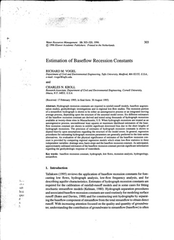
,,,,'.(\j "J)310.;,.,cf;.RICHARD M. VOGEL AND CHARLES N. KROLL1.0. .0.90K0.80b 7 Kbi §§ OOO - §0!Ivv"".§i0.6Site# 16m 125!i0.510Fig. I.squares2030 iRECESSION LENGTH, daysEstimatesof Kb for 125hydrographrecessionsat site 16 using unconditionalleast(ULS)estimatorsof / , and / 2in Equation(8).Box and Jenkins (1976, pp. 212-236) recommend the use of unconditionalleast squares (ULS) estimators for fitting ARMA models. For very large samples,perhaps 500 or more observations, the ULS estimates are approximately equalto the maximum likelihood estimates. While ULS estimates of the parameters ofan ARMA model are asymptotically unbiased and have minimum variance, theycontain substantial downward bias for the small samplesencounteredhere. Typicalhydrograph recessions encountered in this study ranged from about 6-35 days.For example, Figure 1 contains m 125 independent estimates of Kb at site 16obtained by application of ULS estimators for the AR(2) model parameters i and 2 in (8). Clearly the value of the estimates depend significantly upon the recessionlength, which is not the case for the estimators which follow. For example, twoestimators of Kb described later on reveal that for this site, Kb is in the range [0.900.94]. Clearly each of the m 125 independent ULS estimates of Kb illustrated inFigure 1 are downward biased, and the bias does not disappear completely, evenfor the longer hydrograph recessions.For the AR(1) model in (3) a method-of-moments estimate of the parameterKb is equal to an estimate of the first-order serial correlation coefficient PI, whichis also significantly downward biased for the samples encountered in this study(see Wallis and O'Connell, 1972). Furthermore, the unbiased estimators of Pirecommended by Wallis and O'Connell (1972) are significantly downward biasedwhen Pi 0.9 and n 30 as is usually the casein this study. Since the small sampleproperties of even the most efficient estimators of PI, l, and 2 (and, hence, Kb), ,;; :. C'C!i. j,
-' .'t'". r,- ,\I';", '."c"' lr "1 . .ESTIMATION OF BASEFLOW RECESSIONCONSTANTS311contain substantial downward bias for the short and highly autocorrelated samples!encounteredhere,we electedto treat Equations(3), (4); (8) and (9) as regression',- .equations instead of as time-series.4.2. REGRESSIONESTIMATORSFORTHEAR(l), IMA(O,l,O) ANDAR(2) MODELS- Kbl, Kb2, Kb3 AND Kb4If Equations (3), (5), (8) and (9) are treated as regression equations, then one neednot estimate Kb for each of the m individual recessions at a site. Instead, all thesequencesof flows Qt 1, Qt and Qt-l chosen by the automatic hydrograph recession selection algorithm may be combined and fit to (3), (5), (8) and (9) to producea single estimate of Kb for a site. Since such an estimate is based on hundreds ofobservations, the resulting estimates are sure to be statistically significant as longas the model residuals have constant variance and are approximately normally distributed. For the AR(l) model in (3), an ordinary least squaresregression estimateof Kb isKbI L::: ;;;!Qt l Qt n-1Q2 'L,.,t l( 14)twhere n is the total number of consecutive observations obtained for a site usingthe automatic hydrograph recession selection algorithm. Equation (14) is relatedto Knisels (1963) procedure which estimates Kb by plotting consecutive values ofQt l versus Qt and taking Kb as the maximum slope.Treating the IMA(O,l ,0) model in (5) as a regression problem one obtains theordinary least squaresestimatorKb2 exp[ (Yt -Yt-l)] ,(15)where again Yt In(BJ and Yt-l In(Bt-l). Equation (15) provides one of thesimplest possible approachesto estimation of the baseflow recessionconstant.For the AR(2) model multivariate ordinary least squares regression may beemployed to estimate /Jland /J2in (8), however it was found that the resultingmodel residuals were heteroscedastic. We found that Var(E:J was proportional tothe flows. To account for this heteroscedasticity, Equation (8) was rewritten as Qt'j /Jl / 2 Qt 1]t,where now Var(1]t) Var(E:JIQ2hence the residuals 1]t are approximately homoscedastic, and simple ordinary least squaresregressionproceduresmay be employed toestimate /JI and / 2 in (16). Substitution of those estimates of /Jland /J2into (8) and(10) leads to an AR(2) model estimate of Kb which we term Kb3. This procedureis essentially a weighted least squares approach to estimating the residuals in (8)where the weights are proportional to the streamflows. (16)(-
,.,('c\; " .; " l!:&:312RICHARD M" VOGEL AND CHARLES N. KROLLI ';.;When model errors for the AR(2) model are assumedto be additive in log space,., "as in (9), then an iterative least squares approach is required (see Kroll, 1989) whichwe term Kb4 in this study.In summary, the estimators Kbl and Kb3 are the estimators for the AR(I) and.AR(2) models, respectively, when the residuals are assumed to be additive inreal space. The estimators Kb2 and Kb4 correspond to the IMA(O,I,O) and AR(2)models, when the residuals are additive in log space."'{ ;"; "c; "Cc: .,;"4.3.:;":':;:;,.:c","THE ESTIMATOR Kb5 OBTAINED BY TREATING THE WATERSHED AS A LINEARRESERVOIR-c,c""",,'3A steady-state solution to the difference equation in (1a) is "'E\;;4 :l ;!:* );;: ;:f lit;; Q - Q (K )tegtt -.0 .','2"",00." ;",;.:,:;:,-."",";1-"", i' , ;:'1:,(::;:,;"C:,ji"" .;,c """",i1'",.,'-;:(17).where Qo IS the lDlual baseflow and Qt IS the baseflow after t days, and t areindependent errors with zero mean and constant variance. Brutsaert and Nieber(1977) and Vogel and Kroll (1992) show that (3) is a solution to the continuityequationd Vldt I- Q, when the outflow Q from the watershed is linearly relatedto the basin storage V, so that Q - V In(Kb) when inflow I to the watershed is, :,cC:j;;j" 1 1".::; :'".1zero (under low-flow conditions) resulting in the differential equation!;i\ ; q?,, : ;'; ;i"':1; :,;;;1-;. ;.";dQ/dt,,".':t,)C"' "" -n I (K b) Q e.gt( 18)Equation (18) can be applied to observed streamflows by taking logarithms toobtainIn[-dQ/dt]f!fj * :':'?ft( ' ;@;::- ;f i?:; ' c r f,;: 'f, {-"i'" In[Q] tt,(19)cC';';;.g-;"';-" ;[;: ': 'f::c",,. In[-ln[Kb]]where the tt are normally distributed errors with zero mean and constant variance.Vogel and Kroll (1992) use the numerical approximations dQldt Qt - Qt-l and;. c ,:, , ; ,:,,;;,f;:,{. -':;;iiQ (Qt Qt-l)/2:ic:,4fJ; i;; 't Kb5to derive the least squares estimator{ [1L {In[Qt-lm t 1 exp -exp -' 5: \"::'";:"" ';:.:i:!(";:ic'o.':' :0,-;';';,m1- Qt] - In[2(Qt Qt l)]}]},(20)where m is the total number of pairs of consecutive daily streamflows Qt and Qt-lat each site. Essentially Kb5 is an ordinary least squares regression estimator of Kbin (19).4.4.THE TRADmONAL BASEFLOWRECESSIONCONSTANTESTIMATORKb5Taking natural logarithms (17) becomesIn(Qt) In(Qo) In(Kb) t tt(21)hence one would anticipate the natural logarithms of baseflow to be linearly relatedto time, with additive errors in log space.Most introductory textbooks on hydrology.,'r "'J.;-
l0.0;313ESTIMATION OF BASEFLOW RECESSIONCONSTANTSTABLE II. Summary of estimators': 0'.EstimatorExplanationEquationsModel error structureKblKb2Kb3Kb4Kb5AR(I) ModelIMA(O, I ,0)AR(2) ModelAR(2)Linear Modelreservoir(3) (14)(5) (IS)(8) (16)(9) (20)(19)Additive in real spaceAdditive in log spaceAdditive in real spaceAdditivein loglog spacespaceAdditive inKb6Traditional(21)Additive in log spaceadvocate fitting (21) by plotting In(Qt) versus t and taking In(Kb) as the minimumslope corresponding to the baseflow portion of the hydro graph. Such graphicalprocedures are often rather arbitrary, hence Singh and Stall (1971) introduced amore objective approach which selects Kb such that the other component of therecession (Equation (1b» is also linear on semi-log graph paper.In this study, the m candidate hydro graph recessions at each site, selected bythe automatic hydro graph recession selection algorithm are fit to (21) using simpleordinary least squares regression. This leads to m estimates of Kb for a given site.Since ordinary least squares regression produces unbiased estimates of In(Kb) in(21), an estimate of the mean of the m estimates ofKb should be a nearly unbiasedestimate of the true value of Kb at a site as long as m is large. The averagevalue ofm regression estimates of Kb at a site is denoted by Kb6. The six estimators of Kbdescribed in the above section are summarized in Table II.5. Results5.1. STAnsnCAL COMPARISONSOFESTIMATORSFigure 2 contains the m individual estimates of Kb obtained at sites 4, 8, 13 and15 using ordinary least squares estimates of In(Kb) in (21). These four sites arerepresentative of the range of drainage areaslisted in Table I. In addition, the averageof the m individualestimates which we term Kb6are depicted by a solid line at eachsite. Essentially, each circle in Figure 2 representsa single estimate of Kb obtainedusing the traditional estimator which is roughly equivalent to passing a straight linethrough the flow versus time relationship on semi-log graph paper. In contrast withFigure 1, the estimator of Kb appears to be an approximately unbiased estimatorof the average value as evidenced by the fact that the estimates appear to form acone with longer recession lengths giving rise to estimates of Kb which are closerto the mean value. Figure 2 dramatizes the variability of individual estimates of Kbderived from individual hydro graph recessions. Apparently, individual estimatesof Kb derived from a single hydro graph are very poor estimates of the true valueof Kb even for fairly long hydrograph recessions.I"'1t
,, ,(II314.;.;.RICHARD M. VOGEL AND CHAt;. b3N. KROLL1.001.000o.eso.eo.Q00000.9SO.as 0K080000.0.90b0.8S0800SITE 40.8061014182226SITE 8300.80610LENGTHOF HYDROGRAPH1.0008800.9S0Q00088090008S00800800000 00.8SSITE 130.806101418222630LENGTH OF HYDROGRAPHFig. 2.I80 880229:U0.9SK b 0.90001826LENGTHOF HYDROGRAPH1.00014000@O 0080 8000.806SITE 151014182226LENGTHOF HYDROGRAPHEstimatesof Kb for individual hydrographrecessionsat sites4, 8, 13 and 15 usingthe traditional approach described by Equation (24).Table III and Figure 3 compare the six estimators Kbl, Kb2, Kb3, Kb4, KbSand Kb6 summarized in Table II for the 23 U.S. Geological Survey gaged basinssummarized in Table I. These six estimators lead, uniformly, to rather differentestimates of Kb at each site. It appearsthat the estimators exhibit somebias relativeto one another, however it is difficult to evaluate that bias since the true values areunknown here. All four estimators have relatively low variance becauseof the largesamples used.The model residuals associated with the estimators Kb2, Kb4, KbS, and Kb6based on (4), (9), (18) and (21), respectively, were homoscedastic and approximately normally distributed. These four estimators assumethat the model errorsare additive in log space.The model residuals were tested for normality using theprobability plot correlation coefficient test (Vogel, 1986) with a 5% significancelevel. Interestingly, the model residuals associated with the estimators Kbl andKb3, based on (3) and (8), respectively, were not homoscedasticand were not normally distributed. Recall that we attempted to correct for this heteroscedasticityassociated with the estimator Kb3 by using a weighted least squaresestimator. Weconclude that hydro graph recession model errors are additive in log space.Therefore hydrograph recessions are not really autoregressiveprocessesas shown in (3)and (6), instead they more closely resemble an IMA(Q,I,Q) processas in (5) or the.i"'{j ";{,,.",;j';; c';; . . i:- "';;, ;;,.,.
:. "l,r.r(JI,'" I1-J-.ESTIMATION OF BASEFLOW RECESSIONCONSTANTS. .O.K bl0.960.94K b2. 8 .1 2 345.Q0 0i.O. o A00.00A0.A000A0. .0.6 7 8 91011121314151617181920212223SiteFig. 3.K b6. .A.O K b5 .8go.00.86K b4. '8 . .A.O.0 . 0 o.0.68A .iiiA8K b3 Kb 0.92 0.90 315NUillberComparison of estimates of Kb at 23 unregulated U.S. Geological Survey sites inMassachusetts.more complex higher order processgiven in (9) which is no longer a AR(2) processbecause the error structure is multiplicative rather than additive in real space.5.2. PHYSICALSIGNIFICANCEOFESTIMATESOF KbThe baseflow recession constant, K b,is a nondimensional parameter which describesthe rate at which streamflow decreaseswhen the stream channel is recharged bygroundwater. Kunkle (1962), Knisel (1963), Bingham (1986), Vogel and Kroll(1992), Demuth and Hagemann (1994), and others have shown that estimates ofKb are highly correlated with basin geohydrologic parameters.Riggs (1961), Bingham (1986), Voge
Kb Jenkins is the (1976) autoregressive for an AR(I) parameter. process, Kb Using cPl. the James notation and Thompson introduced (1970) by Box deriveand I. I' the baseflow recession curve as an ARMA(I, 1) process with Kb cPl (}l. Of course I - James and Thompson did not call their model an ARMA(I,I) process because in [ ', '.