Transcription
Scenario Analysis Approachfor Operational Risk in Insurance CompaniesAnalýza scénářů operačního rizikav pojišťovnáchMICHAL VYSKOČILAbstractThe article deals with the possibility of calculating the required capital in insurancecompanies allocated to operational risk under Solvency II regulation and the aim of thisarticle is to come up with model that can be use in insurance companies for calculatingoperational risk required capital. In the article were discussed and compared the frequencyand severity distributions where was chosen Poisson for frequency and Lognormal forseverity. For the calculation, was used only the real scenario and data from small CEEinsurance company to see the effect of the three main parameters (typical impact, Worst caseimpact and frequency) needed for building the model for calculation 99,5% VaR by usingMonte Carlo simulation. Article comes up with parameter sensitivity and/or ratio sensitivityon calculating capital. From the database arose two conclusions related to sensitivity wherethe first is that the impact of frequency is much higher in the interval (0;1) than above theinterval to calculated capital and second conclusion is Worst case and Typical Case ratio,where we saw that if the ratio is around 150 or higher the calculated capital is increasingfaster that the ration increase demonstrated on the scenario calculation.Keywordsoperational risk, insurance, scenario analysis, distribution, sensitivityJEL ClassificationC150, G320, is paper has been prepared within the project GS/F1/46/2019 (2020) Developmenttrends in financial markets.AbstraktČlánek se zabývá možností výpočtu požadovaného regulatorního kapitálu v pojišťovnáchpro operační riziko podle nařízení Solventnost II. Cílem tohoto článku je přijít s modelem,který lze v pojišťovnách použít pro výpočet kapitálu alokovaného pro operační riziko.V článku byla diskutována a porovnána rozdělení četnosti a dopadu, kde bylo zvolenoPoissonovo rozdělení pro frekvenci a Lognormální rozdělení pro dopad. Výpočet sezakládá na reálném scénáři a datech z malé pojišťovny ze střední a východní Evropy, abybylo možné pozorovat vliv tří hlavních parametrů (typického dopadu, nejhoršího možnéhodopadu a frekvence), které jsou potřebné pro sestavení modelu pro výpočet na hladině99,5 % VaR pomocí simulace Monte Carlo. Článek přichází s analýzou citlivosti parametrůa / nebo poměrovou citlivostí při výpočtu kapitálu. Z databáze vznikly dva závěry týkajícíACTA VŠFS, 2/2020, vol. 14, www.vsfs.cz/acta153B
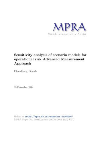
se citlivosti. Dle prvního závěru je dopad frekvence v intervalu (0; 1) mnohem vyšší nežnad intervalem pro vypočtený kapitál. Jako druhý závěr lze vypozorovat, že pokud jepoměr mezi nejhorším možným případem a typickým případem okolo 150 nebo vyšší,vypočtený kapitál roste rychleji než poměrový ukazatel při výpočtu scénáře.Klíčová slovaoperační riziko, pojištění, analýza scénářů, rozdělení, citlivostIntroductionScenario analysis the recurring process of obtaining expert opinion with own operationalevent recorded in company/group to identify and evaluate major potential Operationalrisk events and assess their potential impacts, ensuring a forward-looking risk point ofview (Rippel and Teplý, 2008). From a measurement perspective Scenario Analysis providesa forward-looking cross-functional assessment of the potential size and likelihood ofacceptable operational losses or events and delivers the proper inputs for OperationalRisk capital requirement calculation by using the Internal Model. On the other handfrom a management perspective Scenario Analysis, may start or drive the process ofidentification Operational risks which are existing currently or may potentially appear withimpact to company and control weaknesses, with the purpose of defining and addressingthe risk prevention and their mitigation techniques or strategies. Scenario analysis inbanking industry as a calculating method was mentioned or used in Arai (2006), Mulveyand Erkan (2003), Rosengren (2006) or Dutta (2014) where scenarios had two importantelements: Evaluation of future possibilities and Present knowledge and Dutta (2014) didnot put such emphasis on historical data. Aim of this paper is come up with model basedon three parameters which can be derive from historical data or collected from expertsfrom insurance companies (expert judgement) during meetings and come with issues thatcan arise during parameters collection.1Data and MethodologyAs opposed to banks, insurance companies do not have such a large database ofoperational risk events because they started to deal with the risks later on. For this reason,there is a problem with the data used for both scenario creation and scenario parametersto calculate the capital required. For this reason, it is clear that only data from our ownexperience can not be used and it is necessary to resort more to market data and expertjudgments.154ACTA VŠFS, 2/2020, vol. 14, www.vsfs.cz/acta
Figure 1: Data SourcesType of SourcesForward–LookingHistoricalTime ViewExternalInternal– use consultance– use previous operationalrisk assessments (if they areforeward–looking)– use strategic planning fromsenior management or parentcompany– use operational risk databasefrom the world– buy database from anothercompany or broker– use international loss datadatabase– work with key risk indicators– use audit findings– use parent company databaseSource: AuthorThe problem may arise, in particular, in the use of external resources, because thebusiness and overall set-up or risk appetite of one insurer is not always the same as others,therefore it may threaten other risks, even in the group may be different risk perceptionbetween mother and subsidiary company. This raises another problem with using externaldatabases. Different states face different risks with different impacts, which need to befurther considered and treated with caution. Last but not least, it is necessary to correctlyadjust the weights between the above four quadrants for appropriate setting.2Parameter selectionIt is needed to define two parameters for severity calibration. First is typical impactand second is Worst case. To obtain Typical case as a severity distribution parameterthe parameter has to be matched with a central tendency measure. Common statisticstendencies are mode (most frequent loss), median (loss amount which separates lossesto two halves and expected value (mean, the probability-weighted average of all losses).The main problem with using mode as parameter is in the skewed distribution becausethe mode is matched with small negligible losses and the difference between mode andexpected value can be really significant and this difference becomes larger when thefrequency is increasing. Median has to deal with significant issue when the distribution isnot symmetric and when number of losses is quite low the explanatory value is poor. Onthe other hand expected value is commonly use in statistics and can deal with problemright skewed distribution. All three parameters have problem with Worst Case representsthe worst possible economic impact arises from an operational risk occurrence. The eventshould be considered as an extreme but still realistic scenario on the basis of internalcontrols system, environmental factors (because of lack of big operational risk losses).Frequency is defined as annual expected number of loss and is the only one parameterfor calculation.ACTA VŠFS, 2/2020, vol. 14, www.vsfs.cz/acta155B
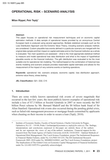
3Severity distributionThe sub-exponential distributions have tails that are descending slower than theexponential distribution (meaning a fatter tail). A fat tailed distribution guaranteesa relevant (higher) level of conservatism and captures the tail behavior of the operationallosses (low frequency but high impact).3.1Lognormal distributionLognormal is a continuous distribution, defined on R , and identified by two parameters,a scale parameter μ and a shape parameter σ.3.2Weilbull distributionWeibull is a continuous distribution, defined on R , and identified by two parameters,a shape parameter k and a scale parameter λ, that are non-negative. This distribution issub-exponential only if the shape parameter is lower than 1.3.3Log logistic distributionLog-logistic is a continuous distribution, defined on R , identified by two parameters, α isthe scale parameter and β is the shape parameter. Distribution is always sub-exponential.3.4Severity distribution quantitative analysisThe main difference between the distributions described above is the (long) tail behavior.Pretty useful graphical tool for analyzing the (long) tail behavior is the survival plot(1-F(x)). The survival plot you can see below shows the tail behavior of the three mentioneddistributions calibrated with the same set of inputs. Weibull distribution presents thefastest tail decay, while the Log-logistic presents the slowest tail decay: given the sameWorst Case the extreme values drawn by the Loglogistic are higher than the extreme valuedrawn from Lognormal, and the extreme values drawn from Lognormal are higher thanthe extreme value drawn from Weibull.156ACTA VŠFS, 2/2020, vol. 14, www.vsfs.cz/acta
Figure 2: Survival Plot for Severity DistributionsSource: AuthorBecause of lack of data in database especially in the long tail the selected distributionwe can not use a goodness of fit test approach. According to the lack of data will beimpossible to select certain distribution that will provide us a conservative figure for eachscenario.3.5Distribution comparisonRelated to lack of enough big dataset we do not truncate the distribution because it isimpossible to detect the certain breaking point. So we decided to apply the one onlydistribution same as authors in the banking industry Shevchenko & Peter (2013), Gatzert& Kobl (2014), Frachot, Georges and Roncalli (2001) or Chernobai (2007) because there isa lack of literature related to insurance industry.The lognormal distribution seems to be the most appropriate distribution to model theseverity from the following points:- The Lognormal distribution allows to apply a prudential approach in line withindustry standards- It has only two parameters (mu and sigma) as compare to other distributionswhere there are three variables- Several studies show that the lognormal is a good choice to model the operationalrisk losses. The literature shows how the Log-Normal is a common distributionused to analyze the Operational risk. In their analysis, Dutta and Perry (2006) cameup with conclusion that Log-Normal distribution produces reasonable capitalestimates for many business lines. In additional the Log-Normal performanceACTA VŠFS, 2/2020, vol. 14, www.vsfs.cz/acta157B
is less complicated with similar results compared with distributions that have3 or 4 parameters as mentioned above. Even Basel Committee used the LogNormal Distribution to fit the results from 2008 Loss Data Collection Exercise forOperational Risk purposes. Basel Committee also confirms that the Log-Normaldistribution is used by banks frequently for various purposes, and that it tends tofit actual loss data well. Cruz (2015), stated that the Log-Normal often give a goodfit for Operational risk losses. Log-Normal distribution is the common distributionused to model the severity in Chernobai et al. (2007).- Survival plot shows that it is not possible to select a priori distribution that isconservative for each scenario due to their diversity. However, since the Log-normaltail behavior is intermediate (between high and low tail heaviness). Log-Normaldistribution is more optimal compared with other sub-exponential distributionbecause the probability of high VaR deviation from probably real distribution isminimized.4Frequency Distribution SelectionFrequency represents the average number of operational risk losses events whoseoccurrence is expected within a on-year time horizon and taking into account experienceof internal resources, skills, business complexity and exposure to environmental factors.Frequency distribution provides information about number of operational lossesoccurrence in certain time period. The distribution is modelled by using a discretedistribution therefore the number of occurrence has to be integer. The frequencyof random events can be likened to a discrete random variable where the number ofpossible observations finite or countable. The most common statistical distributions usedin operational risk models are Binomial, Poisson and Negative Binomial distribution.4.1Binomial distributionBinominal distribution is represented by Bi(n,p) and id a discrete distribution which canbe applied to the frequency’s model part for operational losses in a given interval withn events that has only two outcomes: failure and success with probabilities 1-p and p,respectively (Dyer, G., 2003).The binomial distribution can better fit for modeling count data where the variance is lessthan the mean (Cruz, M, 2002). One major reversal in using the binomial distribution tomodel frequency of operational losses is the assumption of the number of trials (n) in thecalculation (Ross, 2002). This may be the reason why this distribution is not widely used(Klugman, 2004) because the n is unknown. More so, when n is large and p is small, thebinomial distribution can be approximated by a Poisson distribution.158ACTA VŠFS, 2/2020, vol. 14, www.vsfs.cz/acta
4.2Poisson distributionPoisson distribution can be used to model for number of such arrivals that occur ina defined fixed period of time. In operational risk, Poisson process can help in modelingthe frequency of operational losses that is a pre-requisite in estimating the regulatoryoperational VaR. The Poisson distribution is one of the most popular and common usedfrequency estimation because of its simplicity of use (Cruz, 2002). Poisson distribution wasused also for operational risk modelling for LDA (Gatzert, 2014).The most simplistic and attractive property of the Poisson distribution is that only the onlyone parameter lambda is needed to identify both the scale and shape of the distribution.To fit a Poisson distribution the only one step needed is to estimate the mean numberof events in a defined time interval. This distribution is particularly used when the meannumber of operational losses is sort of constant over time.Another property is that the sum of n Poisson distribution with parameters λ1, λ2, λnfollows a Poisson distribution with parameters λ1 λ2 λn.4.3Negative binomial distributionThe negative binomial distribution is a discrete probability distribution of the numberof successes in a sequence of independent and identically distributed Bernoulli trialsbefore a specified (non-random) number of failures (denoted r) occur. In operational riskterminology, the number of failures (n) until a fixed number of successes (r) can comprisethe number of days (n) that elapsed before a fixed number of operational losses (r) wasobserved.The negative binomial distribution is probably the most popular distribution inoperational risk after the Poisson (Cruz, G, 2002) because of it’s two parameters and theadditional parameter offers greater flexibility in the shape of its distribution. This twoparameter property releases the assumption of a constant rate of loss occurrence in overtime assumed by the Poisson. Variance is greater than the mean is another assumption ofthe negative binomial distribution.From information above can be seen that the negative binomial distribution is a specialgeneralized case of the Poisson distribution where the intensity rate λ is no longer constantbut can follow a Gamma distribution with a transformed λ m, k (where m mean, whilek is a measure of dispersion of such distribution). This implies that λ has now been splitinto two parameters to consider the inherent dispersion in the data set which is a placeto refine.ACTA VŠFS, 2/2020, vol. 14, www.vsfs.cz/acta159B
4.4Frequency conclusionParameter sigma (shape) has impact calculating VaR in comparison to parameter mu.When the sigma is increasing the difference between Negative Binominal and Poisson hasdecrease behaviour because if sigma increases the severity distribution tail becomes moreflat. The Negative Binominal distribution is more conservative in comparison to Poissondistribution but only when the frequency is very low and the severity tail is light, thanthe difference is only material. Low sigma and low frequency are connected to scenarioswith the smallest VaR value and their impact is relatively negligible, so the choice of thedistribution has a minimum impact on the overall results.The other main advantages for choosing Poisson distribution compared to otherdistributions are:- Easy to calibrate: Poisson is identified by only one parameter (λ)- Easy to interpret: the λ parameter is interpretable as the average annual frequency- Endorsed by literature: use of Poisson for modeling the frequency is often reportedin literature (Bening & Korolev, 2002; Grandell, 1997; Ross, 2002 and Dutta & Babbel,2014)5Aggregated Loss DistributionWe have decided to use frequency calculated for one year and the probability distributionfunction of the single event severity impact for each risk scenario as under the LossDistribution Approach (LDA). LDA is commonly use in banks compared to insurancecompanies not just because of not enough large databases. Usage of LDA deals withissue that random observation from the severity distribution can be calculated by eitherFourier or Laplace transforms as suggested in Klugman et al. (2004) and used in Dutta& Babbel (2014) by Monte Carlo simulation as they used for banks. We assume implicitlythat the random variables and number of events are both independently distributed sameas in Dutta & Babbel (2014) as they used for banks. We can find LDA approach in Frachot,Antoine and Georges and Roncalli (2001), Schevchenko & Peters (2013) or Wang et al.(2017). Operationally a single random value of the aggregated loss distribution can beobtained using extract a random observation (n) from the Poisson distribution definedby λ for frequency and extract (n) random and independent observations from Lognormaldistribution defined by the μ and δ parameters for severity purposes and we assume thatWorst case happens one time every 100 events. Then we obtain the random observation(i) from aggregated loss distribution as a sum of the (n) random values extracted infrequency and severity step. For computing the aggregated loss distribution we decidedto use Monte Carlo calculated on a 99.5% quantile according to Solvency II purposes.Lognormal distribution and Poisson are chosen because of possible usage in insurancesector where as mentioned above is a lack of historical data and scenario analysis hasto be build up more on expert judgements. That could be serious issue to obtain moredetailed parameters than typical case represented by expected value and Worst case so itis necessary to use simpler approach.160ACTA VŠFS, 2/2020, vol. 14, www.vsfs.cz/acta
6Scenario analysis – Internal fraudIn the tables below you can find stress tests of frequency, typical case (represented byexpected value) and worst case. Scenario analysis represented Internal fraud where theTypical case is 27 000 EUR, WC was estimated by expert judgement to value 359 000 andthe annual frequency is 16.Table 1: Sensitivity Results (Frequency)FrequencyTypical Impact(Severity)Worst Case(Severity)VaR 007,741,911Source: Insurance company database authorial computationTable 2: Sensitivity Results (Typical Impact)FrequencyTypical Impact(Severity)Worst Case(Severity)VaR ,0001,364,785ACTA VŠFS, 2/2020, vol. 14, www.vsfs.cz/acta161B
rce: Insurance company database authorial computationTable 3: Sensitivity Results (Worst Case)FrequencyTypical Impact(Severity)1627,0001616Worst Case(Severity)VaR 41,588,647Source: Insurance company database authorial computation7ConclusionIn this paper we develop model for calculating operational risk on VaR 99.5% as requiredfrom Solvency II directive. This model is based on the selection of Poisson distribution forfrequency with the only one parameter lambda, which is representing the annual lossoccurrence and the selection of Lognormal distribution for severity purposes where weuse two parameters (typical case and Worst case). The biggest advantage of this developedmodel is that every scenario can be calculated by using just three parameters and theparameters cannot be based just on historical losses from database but can reflect theforward-looking scenario nature. On the other hand could be challenge or issue to keepthe expert judgment in proper way and avoid possible biases.162ACTA VŠFS, 2/2020, vol. 14, www.vsfs.cz/acta
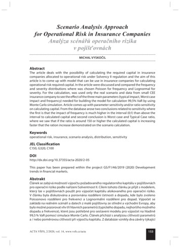
Figure 3: VaR Sensitivity to FrequencySource: AuthorThe Figure 1 shows that the frequency parameter λ has a higher sensitivity and/or impacton the calculated capital at VaR 99.5% in interval (0;1) and then above 25 loss events peryear. We have proved that this method fits to operational risk because of the typical losses,which the company worried about, are happening less than one per year and choosingPoisson distribution for this scenario example is correlating to Bening & Korolev (2002),Grandell (1997), Ross (2002) and Dutta & Babbel (2014).Figure 4: VaR Sensitivity to Worst Case and Typical Case RatioSource: AuthorAs a further interest in the calculations, the ratio between the Worst case scenario and thetypical case scenario arose with focus on VaR sensitivity. From the chart above is obviousACTA VŠFS, 2/2020, vol. 14, www.vsfs.cz/acta163B
that if the typical case is stable (27 k EUR) and Worst case is increasing, the VaR sensitivity isascending related to Worst case to Typical ratio. Except few point the curve VaR sensitivityis slightly increasing the whole time.Although the typical case is, for example, lower than another typical case, the final amountof capital required may be higher due to the large ratio between the Worst case and thetypical case. As we can see from the calculated results above, the typical case is the capitaldriver when the difference between typical case and Worst case in not that high and thevalues are close to each other.After computing all operational risk scenarios we will come across a series of correlationsbetween them. Most of the correlation between the categories of operational risk oroperational risk scenarios, which may not always accurately replicate the structure, willbe based on expert estimates due to a lack of data. The correlation between categories orscenarios cannot be measured every day, as is the case with market risk, and it is thereforevery important to set up correct correlations, which will probably have a major impact onthe final amount of capital required to meet the operational risk requirements.ReferencesARAI, T. (2006). Key points of scenario analysis. Bank of Japan, 2006, http://www.boj.or.jp/en/type/release/zuiji new/data/fsc0608be2.pdfBENING, V. & V. Y. KOROLEV (2002). Generalised Poisson Models and their Applications inInsurance and Finance. Utrecht, Boston: VSP International Publishers.CHERNOBAI, A. (2007). Operational Risk: A guide to Basel ll Capital Requirements, Models,and Analysis. New Jersey: Wiley Finance.CRUZ, PETERS, SHEVCHENKO et al. Fundamental aspects of operational risk andinsurance analytics : a handbook of operational risk. Hoboken, NJ : Wiley; 2015. Available at:http://hdl.handle.net/1959.14/1249294.DUTTA, K. and J. PERRY. A Tale of Tails: An Empirical Analysis of Loss Distribution Models forEstimating Operational Risk Capital. FRB of Boston Working Paper No. 06-13. Available atSSRN: https://ssrn.com/abstract 918880 or http://dx.doi.org/10.2139/ssrn.918880DUTTA, K. & D. BABBEL (2014). Scenario Analysis in the Measurement of Operational RiskCapital: A Change of Measure Approach. The Journal of Risk and Insurance, 81(2), 303–334.Retrieved from http://www.jstor.org/stable/24546806FRACHOT, A., P. GEORGES and T. RONCALLI. Loss Distribution Approach for Operational Risk(March 30, 2001). Available at SSRN: https://ssrn.com/abstract 1032523 or http://dx.doi.org/10.2139/ssrn.1032523GRANDELL, J. (1997). Mixed Poisson Processes. London: Chapman and Hall.GATZERT, N. & A. KOLB (2014). Risk Measurement and Management of Operational Riskin Insurance Companies from an Enterprise Perspective. The Journal of Risk and Insurance,81(3), 683–708. Retrieved from http://www.jstor.org/stable/24548086KLUGMAN, S. Α., H. H. PANJER and G. Ε. WILLMOT (2004). Loss Models: From Data toDecisions. 2nd edition. New York: John Wiley & Sons, Inc.164ACTA VŠFS, 2/2020, vol. 14, www.vsfs.cz/acta
Results from the 2008 Loss Data Collection Exercise for Operational Risk. Bank for InternationalSettlements [online]. Copyright [cit. 29.12.2018]. available at: https://www.bis.org/publ/bcbs160.pdfRIPPEL, M. and P. TEPLÝ (2008). “Operational Risk – Scenario Analysis” IES Working Paper15/2008. IES FSV. Charles University.ROSENBERG, J. V. and T. SCHUERMANN (2004). A General Approach to Integrated RiskManagement with Skewed, Fat-Tailed Risks. Technical report, Federal Reserve Bank of NewYork, 2003, http://papers.ssrn.com/sol3/papers.cfm?abstract id 545802ROSS, S. (2002). Introduction to Probability Models (8th ed.). Boston: Academic Press.SHEVCHENKO, P. V. and G. W. PETERS (2013). Loss Distribution Approach for OperationalRisk Capital Modelling under Basel II: Combining Different Data Sources for Risk Estimation.Journal of Governance and Regulation 2: 33–57.WANG, Y., J. LI and X. ZHU (2017) A Method of Estimating, Operational Risk: LossDistribution Approach with Piecewise-defined Frequency Dependence. Procedia ComputerScience 122, pp. 261–268.Contact addressMichal Vyskočil, Ph.D.candidate at Faculty of Finance and AccountingUniversity of Economics in Prague, Czech Republic(vyskocil.michal@centrum.cz)ACTA VŠFS, 2/2020, vol. 14, www.vsfs.cz/acta165B
153B Scenario Analysis Approach for Operational Risk in Insurance Companies Analýza scénářů operačního rizika v pojišťovnách MICHAL VYSKOČIL Abstract The article deals with the possibility of calculating the required capital in insurance companies allocated to operational risk under Solvency II regulation and the aim of this article is to come up with model that can be use in .