Transcription
Learning Riemannian Metrics for Classification of Dynamical ModelsFabio Cuzzolin and Stefano SoattoDecember 17, 2005AbstractConsider the problem of classifying motions, encoded as dynamical models of a certain class. Standard nearest neighbor classification then reduces to find a suitable distance function in the space of the models. In this paper we present asupervised differential-geometric method to learn a Riemannian metric for a given class of dynamical models in order to improve classification performances. Given a training set of models the optimal metric is selected among a family of pullbackmetrics induced by the Fisher information tensor through a parameterized diffeomorphism. Experimental results concerningaction and identity recognition based on simple scalar features are shown, proving how learning a metric actually improvesclassification rates when compared with Fisher geodesic distance and other classical distance functions.1IntroductionHuman motion recognition is one of the most popular fields in computer vision, due to both its applicative potential andits richness in terms of the technical issues involved. Consider then the problem of classifying a number of movements,represented as sequences of image features: Representing those sequences in a compact way as simple dynamical models hasproved to be effective in problems like dynamic textures or gait identification.The motion classification problem then reduces to finding the appropriate distance function in the space of the dynamicalmodels of the chosen class. A number of distance functions for linear systems has been already introduced, in particular in thecontext of system identification: Martin’s distance between cepstrums [1], subspace angles [2], gap metric [3] and its variantsnu-gap [4] and graph metric [5], kernel methods [6]. Besides, a vast literature can be found about dissimilarity measuresbetween hidden Markov models [7, 8], most of them variants [9] of the Kullback-Leibler divergence [10, 11]. However, asimple mental experiment is enough to understand how no single distance function can possibly outperform the others ineach and every classification problem, since labels can be assigned arbitrarily to any given dataset.The most reasonable thing to do, when possessing some a-priori information in terms of partially labelled data or similarityclasses, is then try and learn in a supervised fashion the “best” distance function for a precise classification problem. Thistopic has become quite popular in the last few years (see for instance [12, 13, 14, 15, 16, 17, 18]). Many unsupervisedalgorithms, in particular, take an input dataset and embed it in some other space, implicitly learning a metric (locally linearembedding [19] among the others), but fail to learn a full metric for the whole input space.In this paper we propose a differential-geometric method that, given a dataset of unlabeled linear systems of a given class,allows to learn the Riemannian metric that minimizes the inverse volume element around the data, this way forcing thegeodesic of the manifold to pass through the region where the data are actually distributed. We will show how this improvesthe classification performance by posing the problem in the region where the systems actually live. More precisely, if themodels belong to a Riemannian manifold M , any diffeomorphism of M onto itself induces a pullback metric on M . Bydesigning a suitable family of diffeomorphisms depending on a parameter p we then obtain a family of pullback metrics onM . We can then analytically compute the volume element of the induced metric as a function of p, and pose a well-definedoptimization problem to get the value of the parameter.To prove the advantages of a classification scheme based on a metric learnt from the data, we consider two differentproblems: action recognition and identity recognition from gait. We use the image sequences collected in the Mobo database[20] to show experiments in which simple nearest-neighbor classifiers based on the pullback of the classical Fisher metricbetween stochastic models outperform analogous classifiers based on all the known distances between models.
2Learning pullback metricsThe study of the geometrical structure of the space formed by a family of probability distribution is first due to Rao [21], andwas developed by Nagaoka and Amari [22, 23]. A family S of probability distributions p(x, ξ) depending on a n-dimensionalparameter ξ can be regarded in fact as an n-dimensional manifold. If the Fisher information matrixh logp(x, ξ) logp(x, ξ) i.gij E ξi ξjis nondegenerate, G [gij ] is a Riemannian tensor, and S is a Riemannian manifold. The squared distance ds2 between twonearby distributions p(x, ξ) and p(x, ξ ξ) is known to be twice the respective Kullback-Leibler divergence [10]. Someapproximations of this measure have been introduced based on Monte-Carlo methods or simplifying approximations [11, 7].The problem of defining a metric for linear dynamical systems has been studied also in the framework of robust control.One criterion is to compare the outputs when the inputs are restricted to the class of inputs that give bounded outputs. Thisapproach was introduced by Zames and El-Sakkary [3] [24] using the notion of gap metric. The original rationale for the(linear) gap metric was to provide a suitable topology in which small errors in the gap in open-loop systems would correspondto small errors in the norm of the stable closed-loop. Another solution called ν-gap metric to the problem of comparing twosystems that is appropriate for feedback analysis was suggested by Vinnicombe [4].Another distance function has recently been introduced based on the notion of cepstrum, the inverse Fourier transform of thelogarithm of the spectral density. Martin [1] defined a new metric for the set of SISO ARMAP models, based on the innerproduct of the cepstra (cn )n Z , c n c n , yielding a Euclidean metric d(c, c0 ) c c0 2 n n cn c0 n 2 . De Cock [2]showed how the cepstrum norm of a SISO ARMA model is a function of the principal angles between the row space of thecontrollability matrices of the model and its inverse.2.1Learning metrics from the data: pullback metricsNone of the above distances (which have usually been designed for a precise goal) can obviosly outperform the others inevery classification problem. Labels can be assigned arbitrarily to dynamical systems, so that a distance which works wellfor a particular labeling would fail if employed in a different classification task. When having some knowledge about thedataset (similarity between pairs, partial labeling, etc.) it makes much more sense to learn a distance metric reflecting thisinformation, and use the learnt metric for classification (see [25]). Many unsupervised algorithms take an input dataset andembed it in some other space, implicitly learning a metric ([19] among the others). However, they fail to learn a full metricfor the whole input space, so that the embedding has usually to be recomputed when new data are available1 .Some simple notions of differential geometry can provide us with a fundamental tool to build a structured family ofmetrics on which to define an optimization problem, the basic ingredient of a metric learning algorithm. Consider a familyof diffeomorphisms between the Riemannian manifold M in which the dataset D M resides and itself:Fλ :M M, m 7 Fλ (m)(1)This family of maps induces a family of pullback metrics on the space itself. Let us call Tm M the tangent space to M in m.Any diffeomorphism F is associated with a push-forward mapF :Tm Mv Tm M 7 TF (m) Mv 0 TF (m) Mdefined as (F v)f v(f F ) for all the smooth functions f on M . Then, given a Riemannian metric g : T M T M Ron M , the diffeomorphism F induces a pullback metric on M as follows:.g m (u, v) gF (m) (F u, F v).(2)Any parametric family of differentiable maps (1) generates naturally a parametric family of metrics on the original space M .The geodesic (shortest path) connecting two points under the pullback metric is the lifting of the geodesic associated with theoriginal metric. In other words, the pullback geodesic between two points is just the geodesic connecting their images withrespect to the original metric.1 Eventhough some work on out-of-sample extensions of spectral methods has been done [26].2
3Volume element minimizationAs our task is to classify data, a natural optimization criterion would be to maximize the classification performance achievedby using the learnt metric for a simple nearest-neighbor classifier. Xing et al. [25] have recently proposed a way to solvethis optimization problem for linear maps y A1/2 x, when some pairs of points are known to be “similar”. This leads toa parameterized family of Mahalanobis distances kx ykA . Given the linearity of the map the problem of minimizing thesquared distance between similar points turns out to be convex, hence solvable with efficient numerical algorithms. Otherpeople [27] have successfully faced the same problem in a linear framework, by solving an optimization problem based oninformation theory (relevant component analysis).Unfortunately, maximizing classification performance is in practice very hard in a nonlinear context. A reasonable approach consists then on choosing a different objective function, which has to be correlated with the natural one in the sensethat it should improve classification performances. An interesting choice has been recently suggested by G. Lebanon [28] inthe context of document retrieval (see also [29]). The idea is to minimize the volume element associated with the pullbackmetric, in order to force the geodesics to pass through the most populated regions of the original space. More precisely, thefunction to minimize is1NY(det g(mk )) 2O(D) .(3)R1(det g(m)) 2 dmk 1 Mwhere g(mk ) denotes the Riemannian metric at the point mk of a dataset living on a Riemannian manifold M . This isclearly related to finding a lower dimensional representation of the dataset, in a similar fashion to dimensionality reductiontechniques like locally linear embedding [19] or laplacian eigenmaps [30]2 . The function (3) to optimize can also be seen asthe inverse of Jeffreys’ prior [31, 28].3.1AlgorithmTo find the expression of the Gramian det g associated with the pullback metric (2) we first need to choose a base of thetangent space Tm M to M . Let us then denote with { i }, i 1, ., dim M the base of Tm M . We can then compute thepush-forward of the vectors of this base, getting in turn a base for TF (m) M . By definition [32], the push-forward of a vectorv Tm M is . dFp (v) dtFp (m t · v) t 0 , v Tm M.(4).The diffeomorphism Fp then induces a base for the space of vector fields on M , wi {Fp ( i )}, for i 1, ., dim M . Wecan rearrange these vectors as rows of a matrix J [w1 ; · · · ; wdim M ]. The volume element of the pullback metric g in apoint m M is then given by the determinant of the Gramian [28],.det g (m) det[g(F p ( i ), F p ( j ))]ij det(J T gJ).If J is a square matrix (as in the following) we get simplydet g (m) det(J)2 · det g(m).We can then easily find the expression of the objective function (3). Of course, once found the optimal metric, standardclassification algorithms require to measure the geodesic distance between any two points. As geodesics for g p are liftings,we only need to know the geodesics of the original Riemannian space.4Learning metrics for linear dynamical modelsEven though large classes of non-linear models can be endowed with a Fisher metric tensor, most efforts have focused on therelatively simpler task of analyzing the Fisher geometry of some important classes of linear models [33, 34]. In particular,the analytic expressions of the entries of the Fisher information matrix for several manifolds of linear MIMO systems havebeen discovered by Hanzon et al. [35].Let us consider first the class of stable autoregressive discrete-time processes of order 2, AR(2), in a stochastic settingin which as before the input signal is a Gaussian white noise with zero mean and unit variance. This set can be given a2 In[30] in particular, dimensionality reduction is considered a factor in improving classification.3
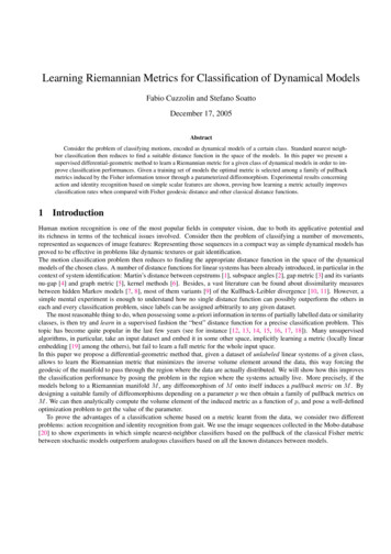
Riemannian manifold structure under Fisher metric [36]. A natural parametrization uses the non-unit coefficients (a1 , a2 )of the denominator of the transfer function, h(z) z 2 /(z 2 a1 z a2 ) (which corresponds to the AR difference y(k) a1 y(k 1) a2 y(k 2)). To impose stability the necessary conditions are1 a1 a2 0,1 a1 a2 0,1 a2 0.The manifold is then composed by a single connected component (see Figure 1). The Riemannian Fisher tensor can beexpressed as [37]µ¶11 a2a1g(a1 , a2 ) .(5)a11 a2(1 a1 a2 )(1 a1 a2 )(1 a2 )However, alternative local coordinates are given by the Schur parameters γ1 a1 /(1 a2 ), γ2 a2 under which the metrictensor simplifies asÃ!(1 γ2 )2102(1 γ1 )g(γ1 , γ2 ) (6)(1 γ22 )01while the parameter domain becomes γ1 1, γ2 1.a2[-2,1][2,1]aa1[0,-1]Figure 1: Graphical representation of the manifold of stable autoregressive systems of order 2, AR(2), with the non-unitcoefficients of the denominator of h(z) as parameters. It forms a simplex with vertices [ 2, 1], [2, 1], [0, 1].Consider now the class of stable discrete-time linear SISO systems of order 1,½x(k 1) ax(k) bu(k)y(k) cx(k)(7)for which we can choose a canonical representation by setting c 1, so that the transfer function is h(z) b/(z a). Wedenote this class of systems with M (1, 1, 1). Under the conditions a 1 (stability) and b 6 0 (minimality) this family oflinear models form a manifold with local coordinates (a, b), consisting of the two connected components {(a, b) : a 0, b .b0} and {(a, b) : a 0, b 0}. Using the generalized polar coordinates r 1 a, θ atanh(a) the Fisher tensor becomes2µ¶1 0g(r, θ) (8)0 r2and the manifold M (1, 1, 1) coincides with the two-dimensional plane, vertical axis excluded (r 6 0).4.1GeodesicsWe can use the analytic expressions of the Fisher metric to write the geodesic equations for these classes of linear systems.Using Einstein’s notation the geodesic equation readsddd2 ax Γabc xb xc 02dtdt dt4
where {Γabc } are the Christoffel coefficients of the second kind [32], Γabc Γbcd g ad where g ad g 1 (a, d) are the entries ofthe inverse of the metric tensor, and the Christoffel coefficients of the first kind are a function of the derivatives of the metric:ddd. 1Γabc g ad ( c gbd b gcd d gcb ).2dxdxdxRavishanker [38] has explicitly computed the expression for the Fisher metric of ARMA(p,q) systems using as parametrization the inverses of poles and zeros, and we could then solve the geodesic differential equation analytically.However, all the geodesics of stable AR(2) systems endowed with the Fisher metric (6) as a function of the Schur parameters have been analytically computed by Rijkeboer [39, 36].The analytical expressions of the geodesics of the manifold M (1, 1, 1) endowed with the Riemannian tensor induced by thescalar product of a Hilbert space H2 have been instead computed by Hanzon [40] through an isometry with a Riemanniansurface. We will use it instead of the Fisher tensor in the following3 . More precisely, given two systems Σ1 (r1 , θ2 ) andΣ2 (r2 , θ2 ) their geodesic distance according to the metric (8) isd(Σ1 , Σ2 ) (r12 2r1 r2 cos(θ2 θ1 ) r12 )1/2if θ1 θ2 π and sgn(r1 ) sgn(r2 );d(Σ1 , Σ2 ) r1 r2 otherwise.4.2Volume elements of pullback metrics for spaces of linear modelsThe algorithm of Section 3.1 adapts easily to the case in which the dataset is a collection of linear systems.One natural choice for a diffeomorphism of AR(2) onto itself is suggested by the simplicial form of the manifold (seeFigure 1),1Fp (m) Fp ([m1 , m2 , m3 ]) [λ1 · m1 , λ2 · m2 , λ3 · m3 ](9)λ·mwhere p λ [λ1 , λ2 , λ3 ] with λ1 λ2 λ3 1, while m [m1 , m2 , m3 ] collects the simplicial components of a systema in the manifold:a [a1 , a2 ]0 m1 [0, 1]0 m2 [2, 1]0 m3 [ 2, 1]0 , a AR(2).(10)Theorem 1 The volume element of the pullback metric on AR(2) induced by the diffeomorphism (9) is given bydetg p (m) 1(λ1 λ2 λ3 )2·.(λ · m)6 m21 m2 m3Let us choose as base of the tangent space in AR(2) the set 1 [1/2, 1/2]0 , 2 [ 1/2, 1/2]0 . To compute the Gramianwe need to express the diffeomorphism with respect to a. From Equation (10) a1 2(m2 m3 ), a2 m2 m3 m1 ,2while the inverse relation is m2 1 a41 a2 , m3 1 a41 a2 , m1 1 a2 . Hence Fλ can be expressed in terms of a1 , a2 asFλ (a) 1 [2λ2 (1 a1 a2 ) 2λ3 (1 a1 a2 ), λ2 (1 a1 a2 ) λ3 (1 a1 a2 ) 2λ1 (1 a2 )]0where 2λ1 (1 a2 ) λ2 (1 a1 a2 ) λ3 (1 a1 a2 ), so thatFλ (a tv) [2λ2 (1 a1 tv1 a2 tv2 ) 2λ3 (1 a1 tv1 a2 tv2 ),λ2 (1 a1 tv1 a2 tv2 ) λ3 (1 a1 tv1 a2 tv2 ) 2λ1 (1 a2 tv2 )]0 . dWe can then compute4 dtFλ (m t · v) t 0 , and in particular dFλ (m t · 1 ) t 0 [2λ1 λ2 (3 a2 a1 ) 2λ3 (2λ2 λ1 )(1 a1 a2 ),w1 dt2λ1 λ2 (3 a2 a1 ) 2λ1 λ3 (1 a1 a2 )]3 The4 Therelated geometries have indeed much in common, [40].straightforward details are neglected to improve the readability of the proof.5
whilew2 ddt Fλ (m t · 2 ) t 0 [ 2λ1 λ3 (3 a2 a1 ) 2λ2 (λ1 2λ3 )(1 a1 a2 ),2λ1 λ3 (3 a2 a1 ) 2λ1 λ2 (1 a1 a2 )].The determinant of the matrix J is then (after a few passages)det J 32λ1 λ2 λ31 λ1 λ2 λ3 . 32 (λ · m)3Eventually, the function (3) to maximize assumes the formNYO(p) Rk 1(λ · mk )3 (λ · m)3 m1 m2 m3 dmAR(2)Zwhere the normalization factor(11) (λ · m)3 m1 m2 m3 dmI(λ) AR(2)forbids trivial solutions in which the volume element is minimized by shrinking the whole space. It can be computed bydecomposing the cube (λ · m)3 using Tartaglia’s formula, obtainingXI(λ) c1 c2 c3Z3Y3!c1/2 c2 1/2 a31dm.m3λj jm2m1 c1c!c!c!123AR(2) 3j 1About M (1, 1, 1), Henon’s map is the simplest non-trivial diffeomorphism of the plane: x0 y x2 a, y 0 bx. Herewe choose a modified version:Fp (r, θ) [ bθ ar2 br, br aθ2 bθ ],(12)with p [a, b].Theorem 2 The volume element of the pullback metric on M (1, 1, 1) induced by the diffeomorphism (12) is given bydetg p (x) 4a2 (2arθ br bθ)2 r2 .It is easy to realize that in this case·J 2ar bbb2aθ b so that det J 2a(2arθ br bθ), while from Equation (8) det g(r, θ) r2 .This time the function (3) can be expressed asO(D) Yk11·rk (2ark θk ) brk bθk I(a, b)(13)where I(a, b) is again the normalization factor. Note that when I(p) is hard to compute, or the original manifold has no finitePNvolume (and hence does not admit Jeffrey’s prior), an acceptable replacement is I(p) k 1 (detg(x)) 1/2 .The functions (11) and (7) can be maximized by means of any numerical optimization scheme, simple (like gradientdescent) or more sophisticated.5Human motion experimentsTo test the effectiveness of the approach we considered a significant vision application, namely the recognition of actionsand identities from image sequences. We used the Mobo database [20], a collection of 600 image sequences of 25 peoplewalking on a treadmill in four different variants (slow walk, fast walk, walk on a slope, walk carrying a ball), seen from 66
different viewpoints corresponding to cameras equally distributed around the subject (see Figure 2-left). Each sequence ofthe database possesses three labels: action, view, and identity.The database comes already with preprocessed silhouettes of the moving body as black and white images. As the resultsof the above sections concern only single input-single output linear systems, we chose to extract from each image the widthof the minimum box containing the silhouette. This way, each image sequence is represented as a scalar signal. Each scalarsequence has been then passed as input to an identification algorithm: we hence generated a dataset of linear systems of thetwo classes discussed above, one system for each labeled motion sequence.This metric learning approach is based on the assumption that the two optimization problems, i.e. maximizing classification performance and minimizing volume elements are indeed correlated. We empirically evaluated the goodness of thisconjecture by measuring the performance of a nearest-neighbor classifier based on the optimal pullback metrics induced bythe diffeomorphisms (12), (9), and comparing the results with those of NN classifiers based on all the other known distances(included the Fisher geodesic distance).0.250.20.150.10.0501234567Figure 2: Left: location and orientation of the six cameras in the Mobo experiment (the origin of the frame is roughly inthe position of the walking person on the treadmill). Right: Performance of NN classifier based on all the known distancesbetween dynamical models, included the pullback metric induced by the Fisher geometry. Correct classification rate for theused metrics averaged on the size of the training set, in the ID experiment. 1 - Frobenius norm of the matrices in canonicalform; 2 - gap metric; 3- ν-gap matric; 4 - subspace angles; 5 - basis Fisher metric; 6 - pullback metric with diffeomorphism(14); 7 - pullback metric with diffeomorphism (9).5.0.1Identity recognitionIn a first experiment we selected a training set of models, and used the pullback geodesic distance to classify the identityof the person appearing in a different set of randomly selected sequences. This is a very difficult problem, as there are 25different people, and the one-dimensional signal we chose to represent sequences clearly provides insufficient information.However, measuring the comparative performance of the metrics can be useful to see how learning a metric appositively givesan advantages when using a NN classifier. We implemented a naive Frobenius norm of the system matrices in canonical form,gap and ν-gap metrics [3, 4], subspace angles [2, 1], and of course the Fisher geodesic distance together with the associatedoptimal pullback metric.Figure 2-right shows the percentage of correctly classified testing systems over several runs in which we randomly selectedan increasing number of systems in both training and testing set. We also tested a different diffeomorphism for AR(2) systems,namelyFλ (m) [ λm1 (1 λ)m2 , λm2 (1 λ)m3 , λm3 (1 λ)m1 ],(14)with 0 λ 1. We can notice how the other distances do not show any significantly different behavior. This of course wasto expect, since they have not been designed to solve classification tasks (usually for identification purposes). This has beenthe case in all our experiments. Hence, in the following we will only report the performance of the second best distance forcomparison.7
5.0.2Action 33030202120210101000.640.30.620.20.60.10.5800.56 e 3: Top: Recognition performance of second-best distance (left) and optimal pullback metric for AR(2) systemsand diffeomorphism (14) (right) in the action recognition experiment. Here the whole dataset was considered, regardlessof the viewpoint. Increasing x indices (1 : 50) mean decreasing size of the testing set. Increasing y indices (1 : 5)represent increasing size of the training set. Bottom-left: Difference between the two performances. Bottom-right: relativeperformances for view 5 only. Again, the pullback metric outperforms the best competitor.In a second experiment, we selected a training set of models, and used the pullback geodesic distance to classify the actionperformed by the person in a different set of randomly selected sequences. Recall that all the actions in the Mobo database arejust slightly different variations of the walking gait, and we were using a single scalar feature. Figure 3 illustrates the relativeperformances of the optimal pullback metric for autoregressive systems under deformation map (14) and its best competitor.The correct classification rate has been measured for different sizes of both training and testing set, by randomly selecting foreach class of action an equal increasing number of systems to build the two collections. To test the approach more thoroughlywe also conducted six separate experiments by selecting the portion of the dataset associated with a single view, for eachpossible view. These are completely different classification problems, as the datasets can turn out to live in different submanifolds. It is in fact interesting to try and see what happens when we choose a different class of diffeomorphisms. Figure4 illustrates the average performance of the classifiers associated with the optimal pullback metric for AR(2) models with(this time) diffeomorphism (9) and the best competing distance for four view-dependent experiments. This time increasingabscissae (from 1 to 7) mean an increased testing set size. As usual the average is computed by repeated random selections,and the optimal metric performs far better than the others.Of course the choice of the family of deformations affects the range of candidate metric tensors the algorithm can selectfrom. We have seen as a matter of fact how the first family of mappings, which depends on 2 parameters instead of 1,8
60.450.550.40.50.350.45123456712345671234567Figure 4: Correct action classification rates for four different viewpoints. Sequences are represented as autoregressive order2 systems. The performance (in red) of the pullback metric associated with the map (9) is shown outperforming the bestcompetitor (in blue) for increasing sizes of the testing set.produces a much wider selection choice for the optimization algorithm, eventually delivering a better performance. The samephenomenon can be appreciated in the identity experiment (see Figure 2).It is really interesting to understand whether the size of the training set we use to learn the optimal metric has or notan influence on the classification performance. Of course, as our method exploits the training set to understand the localstructure of the data, it is reasonable to conjecture that larger training sets should lead to better recognition rates, as longas the training data better represent the whole dataset. This is confirmed by Figure 5, where the recognition rate is plottedagainst the size of the training set. Finally, let us visualize the effect of the optimal diffeomorphism on the dataset. We caneasily do it in the action recognition experiment, as there are only 4 labels. Figure 6-left shows an instance of the originaldataset represented as a set of points in the AR(2) simplex. Points of the training set are drawn as squares, while systemsin the testing set are represented as crosses. Figure 6-right shows how the diffeomorphism deforms the space, plotting theimages of the dataset according to the optimal map. Data-points are colored according to their true class. We can visuallyappreciate how the deformation improves the separation between clusters.6ConclusionsIn this paper we discussed the problem of learning the “best” metric for a classification problem involving linear dynamicalmodels. Given a training set of models we pose a related optimization problem in which the pullback metric induced by adiffeomorphism which minimizes the volume element around the available data is learned. We adopt as basis metric tensorthe classical Fisher information matrix. This yields a global embedding, while usual spectral methods only provide imagesof training points.We have also shown experimental results concerning identity and action recognition, which proved how such a learntmetric actually improves classification performance with respect to the Fisher metric and all the other known distancesbetween dynamical models. Setting and solving the minimization problem for MIMO systems is the next natural step. This9
6789Figure 5: Effect of the size of the training set on the recognition accuracy in the action recognition experiment, M (1, 1, 1)systems. As the size of D increases (abscissa indices) the number of correct matches grows in both the overall experimentfor all view (left) and for view 2 (right).0.920.150.90.10.880.050.8600.84 0.050.82 0.1 0.4 0.3 0.2 0.100.10.2 1.7 1.65 1.6 1.55 1.5Figure 6: Effect of the optimal diffeomorphism (9) on the dataset.will be of course of paramount importance to test this approach in a more realistic scenario.References[1] Martin, R.J.: A metric for ARMA processes. IEEE Transactions on Signal Processing 48(4) (April 2000) 1164–11701, 2, 7[2] Cock, K.D., Moor, B.D.: Subspace angles and distances between arma models. Systems and Control Letters (2002) 1,2, 7[3] Zames, G., El-Sakkary, A.K.: Unstable systems and feedback: The gap metric. In: Proc. 18th Allerton Conference onCommunications, Control, and Computers. (Urbana, IL, October 1980) 380–385 1, 2, 7[4] Vinnicombe, G.: A ν-gap distance for uncertain and nonlinear systems. In: Proceedings of the 38th IEEE CDC.(Phoenix, AZ, 1999) 1, 2, 7[5] Vidyasagar, M.: The graph metric for unstable plants and robustness estimates for feedback stability. AC 29 (1984)403–417 110
[6] Smola, A., Vishwanathan, S.: Hilbert space embeddings in dynamical systems. In: Proceedings of the 13th IFACsymposium on system identification. (August 2003) 760 – 767 1[7] Silva, J., Narayanan, S.: Average divergence distance as a statistical discrimination measure for hidden Markov models.Submitted to IEEE Transactions on Speech and Audio Processing (2004) 1, 2[8] Lyngso, R.B., Pedersen, C.N.S., Nielsen, H.: Metrics and similarity measures for hidden Markov models. In: Proceed
Learning Riemannian Metrics for Classification of Dynamical Models Fabio Cuzzolin and Stefano Soatto December 17, 2005 Abstract Consider the problem of classifying motions, encoded as dynamical models of a certain class. Standard nearest neigh-bor classification then reduces to find a suitable distance function in the space of the models.