Transcription
MLSeq: Machine Learning Interface to RNA-SeqData†Dincer Goksuluk1 , Gokmen Zararsiz1 , Selcuk Korkmaz2 , Vahap Eldem3 , AhmetOzturk1 , Ahmet Ergun Karaagaoglu4 and Bernd Klaus51Erciyes University, Faculty of Medicine, Department of Biostatistics, Ankara, TURKEY2Trakya University, Faculty of Medicine, Department of Biostatistics, Edirne, TURKEY34Istanbul University, Faculty of Science, Department of Biology, Istanbul, TURKEYHacettepe University, Faculty of Medicine, Department of Biostatistics, Kayseri, TURKEY5EMBL Heidelberg, Heidelberg, GermanyApril 26, 2022NOTE: MLSeq has major changes from version 1.20.1 and this will bump following versions to 2.y.z inthe next release of Bioconductor (ver. 3.8). Most of the functions from previous versions were changedand new functions are included. Please see Beginner’s Guide before continue with the analysis.AbstractMLSeq is a comprehensive package for application of machine-learning algorithms in classification ofnext-generation RNA-Sequencing (RNA-Seq) data. Researchers have appealed to MLSeq for variouspurposes, which include prediction of disease outcomes, identification of best subset of features (genes,transcripts, other isoforms), and sorting the features based on their predictive importance. Using thispackage, researchers can upload their raw RNA-seq count data, preprocess their data and perform awide range of machine-learning algorithms. Preprocessing approaches include deseq median ratio andtrimmed mean of M means (TMM) normalization methods, as well as the logarithm of counts per million reads (log-cpm), variance stabilizing transformation (vst), regularized logarithmic transformation(rlog) and variance modeling at observational level (voom) transformation approaches. Normalizationapproaches can be used to correct systematic variations. Transformation approaches can be used tobring discrete RNA-seq data hierarchically closer to microarrays and conduct microarray-based classification algorithms. Currently, MLSeq package contains 90 microarray-based classifiers includingthe recently developed voom-based discriminant analysis classifiers. Besides these classifiers, MLSeqpackage also includes discrete-based classifiers, such as Poisson linear discriminant analysis (PLDA)and negative binomial linear discriminant analysis (NBLDA). Over the preprocessed data, researcherscan build classification models, apply parameter optimization on these models, evaluate the modelperformances and compare the performances of different classification models. Moreover, the classlabels of test samples can be predicted with the built models. MLSeq is a user friendly, simple andcurrently the most comprehensive package developed in the literature for RNA-Seq classification. Tostart using this package, users need to upload their count data, which contains the number of readsmapped to each transcript for each sample. This kind of count data can be obtained from RNASeq experiments, also from other sequencing experiments such as ChIP-sequencing or metagenomesequencing. This vignette is presented to guide researchers how to use this package.MLSeq version: 2.14.0Contents1 Introduction21
2 Preparing the input data23 Splitting the data34 Available machine-learning models45 Normalization and transformation56 Model building6.1 Optimizing model parameters . . . . . . . . . . . . . . . . . . . . . . . . . . . . . . . . . .6.2 Defining control list for selected classifier . . . . . . . . . . . . . . . . . . . . . . . . . . . .6677 Predicting the class labels of test samples98 Comparing the performance of classifiers109 Determining possible biomarkers using sparse classifiers1210 Updating an MLSeq object using update10.1 Transitions between continuous, discrete and voom-based classifiers . . . . . . . . . . . . .121411 Session info151IntroductionWith the recent developments in molecular biology, it is feasible to measure the expression levels ofthousands of genes simultaneously. Using this information, one major task is the gene-expression basedclassification. With the use of microarray data, numerous classification algorithms are developed andadapted for this type of classification. RNA-Seq is a recent technology, which uses the capabilities ofnext-generation sequencing (NGS) technologies. It has some major advantages over microarrays suchas providing less noisy data and detecting novel transcripts and isoforms. These advantages can alsoaffect the performance of classification algorithms. Working with less noisy data can improve the predictive performance of classification algorithms. Further, novel transcripts may be a biomarker in relateddisease or phenotype. MLSeq package includes several classification algorithms, also normalization andtransformation approaches for RNA-Seq classification.In this vignette, you will learn how to build machine-learning models from raw RNA-Seq count data.MLSeq package can be loaded as below:library(MLSeq)2Preparing the input dataMLSeq package expects a count matrix that contains the number of reads mapped to each transcript foreach sample and class label information of samples in an S4 class DESeqDataSet.After mapping the RNA-Seq reads to a reference genome or transcriptome, number of reads mappedto the reference genome can be counted to measure the transcript abundance. It is very important thatthe count values must be raw sequencing read counts to implement the methods given in MLSeq. Thereare a number of functions in Bioconductor packages which summarizes mapped reads to a count dataformat. These tools include featureCounts in Rsubread [1], summarizeOverlaps in GenomicRanges [2]and easyRNASeq [3]. It is also possible to access this type of count data from Linux-based softwares ashtseq-count function in HTSeq [4] and multicov function in bedtools [5] softwares. In this vignette, wewill work with the cervical count data. Cervical data is from an experiment that measures the expressionlevels of 714 miRNAs of human samples [6]. There are 29 tumor and 29 non-tumor cervical samples andthese two groups can be treated as two separate classes for classification purpose. We can define the file2
path with using system.file:filepath - system.file("extdata/cervical.txt", package "MLSeq")Next, we can load the data using read.table:cervical - read.table(filepath, header TRUE)After loading the data, one can check the counts as follows. These counts are the number of mappedmiRNA reads to each transcript.head(cervical[ ,1:10]) # Mapped counts for first 6 features of 10 subjects.##############N1N2N3N4N5 N6 N7N8N9N10let-7a 865 810 5505 6692 1456 588 9 4513 1962 10167let-7a*312307362 0 19910173let-7b 975 2790 4912 24286 1759 508 33 6162 1455 18110let-7b* 151827119113 0 11617233let-7c 828 1251 2973 6413 713 339 23 2002 476 3294let-7c*000100 0303Cervical data is a data.frame containing 714 miRNA mapped counts given in rows, belonging to58 samples given in columns. First 29 columns of the data contain the miRNA mapped counts of nontumor samples, while the last 29 columns contain the count information of tumor samples. We need tocreate a class label information in order to apply classification models. The class labels are stored ina DataFrame object generated using DataFrame from S4Vectors. Although the formal object returnedfrom data.frame can be imported into DESeqDataSet, we suggest using DataFrame in order to preventpossible warnings/errors during downstream analyses.class - DataFrame(condition factor(rep(c("N","T"), c(29, 29))))class############################3DataFrame with 58 rows and 1 columncondition factor 1N2N3N4N5N.54T55T56T57T58TSplitting the dataWe can split the data into two parts as training and test sets. Training set can be used to build classification models, and test set can be used to assess the performance of each model. The ratio of splitting3
data into two parts depends on total sample size. In most studies, the amount of training set is takenas 70% and the remaining part is used as test set. However, when the number of samples is relativelysmall, the split ratio can be decreased towards 50%. Similarly, if the total number of samples are largeenough (e.g 200, 500 etc.), this ratio might be increased towards 80% or 90%. The basic idea of definingoptimum splitting ratio can be expressed as: ‘define such a value for splitting ratio where we have enoughsamples in the training and test set in order to get a reliable fitted model and test predictions.’ For ourexample, cervical data, there are 58 samples. One may select 90% of the samples (approx. 52 subjects)for training set. The fitted model is evantually reliable, however, test accuracies are very sensitive tounit misclassifications. Since there are only 6 observations in the test set, misclassifying a single subjectwould decrease test set accuracy approximately 16.6%. Hence, we should carefully define the splittingratio before continue with the classification models.library(DESeq2)set.seed(2128)# We do not perform a differential expression analysis to select differentially# expressed genes. However, in practice, DE analysis might be performed before# fitting classifiers. Here, we selected top 100 features having the highest# gene-wise variances in order to decrease computational cost.vars - sort(apply(cervical, 1, var, na.rm TRUE), decreasing TRUE)data - cervical[names(vars)[1:100], ]nTest - ceiling(ncol(data) * 0.3)ind - sample(ncol(data), nTest, FALSE)# Minimum count is set to 1 in order to prevent 0 division problem within# classification models.data.train - as.matrix(data[ ,-ind] 1)data.test - as.matrix(data[ ,ind] 1)classtr - DataFrame(condition class[-ind, ])classts - DataFrame(condition class[ind, ])Now, we have 40 samples which will be used to train the classification models and have remaining 18 samples to be used to test the model performances. The training and test sets are stored in aDESeqDataSet using related functions from DESeq2 [7]. This object is then used as input for MLSeq.data.trainS4 DESeqDataSetFromMatrix(countData data.train, colData classtr,design formula( condition))data.testS4 DESeqDataSetFromMatrix(countData data.test, colData classts,design formula( condition))4Available machine-learning modelsMLSeq contains more than 90 algorithms for the classification of RNA-Seq data. These algorithms includeboth microarray-based conventional classifiers and novel methods specifically designed for RNA-Seq data.These novel algorithms include voom-based classifiers [8], Poisson linear discriminant analysis (PLDA) [9]and Negative-Binomial linear discriminant analysis (NBLDA) [10]. Run availableMethods for a list ofsupported classification algorithm in MLSeq.4
5Normalization and transformationNormalization is a crucial step of RNA-Seq data analysis. It can be defined as the determination andcorrection of the systematic variations to enable samples to be analyzed in the same scale. These systematic variations may arise from both between-sample variations including library size (sequencing depth)and the presence of majority fragments; and within-sample variations including gene length and sequencecomposition (GC content). In MLSeq, two effective normalization methods are available. First one isthe “deseq median ratio normalization”, which estimates the size factors by dividing each sample by thegeometric means of the transcript counts [7]. Median statistic is a widely used statistics as a size factorfor each sample. Another normalization method is “trimmed mean of M values (TMM)”. TMM firsttrims the data in both lower and upper side by log-fold changes (default 30%) to minimize the log-foldchanges between the samples and by absolute intensity (default 5%). After trimming, TMM calculates anormalization factor using the weighted mean of data. These weights are calculated based on the inverseapproximate asymptotic variances using the delta method [11]. Raw counts might be normalized usingeither deseq-median ratio or TMM methods.After the normalization process, it is possible to directly use the discrete classifiers, e.g. PLDA andNBLDA. In addition, it is possible to apply an appropriate transformation on raw counts and bring thedata hierarchically closer to microarrays. In this case, we can transform the data and apply a largenumber of classifiers, e.g. nearest shrunken centroids, penalized discriminant analysis, support vectormachines, etc. One simple approach is the logarithm of counts per million reads (log-cpm) method, whichtransforms the data from the logarithm of the division of the counts by the library sizes and multiplicationby one million (Equation 1). This transformation is simply an extension of the shifted-log transformationzij log2 xij 1. xij 0.56 10(1)zij log2X.j 1Although log-cpm transformation provides less-skewed distribution, the gene-wise variances are stillunequal and possibly related with the distribution mean. Hence, one may wish to transform data intocontinuous scale while controlling the gene-wise variances. Anders and Huber [12] presented variancestabilizing transformation (vst) which provides variance independent from mean. Love et al. [7] presentedregularized logarithmic (rlog) transformation. This method uses a shrinkage approach as used in DESeq2paper. Rlog transformed values are similar with vst or shifted-log transformed values for genes with highercounts, while shrunken together for genes with lower counts. MLSeq allows researchers perform one oftransformations log-cpm, vst and rlog. The possible normalization-transformation combinationsare: deseq-vst: Normalization is applied with deseq median ratio method. Variance stabilizing transformation is applied to the normalized data deseq-rlog: Normalization is applied with deseq median ratio method. Regularized logarithmictransformation is applied to the normalized data deseq-logcpm: Normalization is applied with deseq median ratio method. Log of counts-per-milliontransformation is applied to the normalized data tmm-logcpm: Normalization is applied with trimmed mean of M values (TMM) method. Log ofcounts-per-million transformation is applied to the normalized data.The normalization-transformation combinations are controlled by preProcessing argument in classify.For example, we may apply rlog transformation on deseq normalized counts by setting preProcessing "deseq-rlog". See below code chunk for a minimal working example.# Support Vector Machines with Radial Kernelfit - classify(data data.trainS4, method "svmRadial",preProcessing "deseq-rlog", ref "T",control trainControl(method "repeatedcv", number 2,5
repeats 2, classProbs TRUE))show(fit)Furthermore, Zararsiz et al. [8] presented voomNSC classifier, which integrates voom transformation [13] and NSC method [14, 15] into a single and powerful classifier. This classifier extends voommethod for RNA-Seq based classification studies. VoomNSC also makes NSC algorithm available forRNA-Seq technology. The authors also presented the extensions of diagonal discriminant classifiers [16],i.e. voom-based diagonal linear discriminant analysis (voomDLDA) and voom based diagonal quadraticdiscriminant analysis (voomDQDA) classifiers. All three classifiers are able to work with high-dimensional(n p) RNA-Seq counts. VoomDLDA and voomDQDA approaches are non-sparse and use all featuresto classify the data, while voomNSC is sparse and uses a subset of features for classification. Notethat the argument preProcessing has no effect on voom-based classifiers since voom transformation isperformed within classifier. However, we may define normalization method for voom-based classifiers using normalize arguement. As an example, consider fitting a voomNSC model on deseq normalized counts:set.seed(2128)# Voom based Nearest Shrunken Centroids.fit - classify(data data.trainS4, method "voomNSC",normalize "deseq", ref "T",control voomControl(tuneLength 20))trained(fit)## Trained model summaryWe will cover trained model in section Optimizing model parameters.6Model buildingThe MLSeq has a single function classify for the model building and evaluation process. This functioncan be used to evaluate selected classifier using a set of values for model parameter (aka tuning parameter )and return the optimal model. The overall model performances for training set are also returned.6.1Optimizing model parametersMLSeq evaluates k-fold repeated cross-validation on training set for selecting the optimal value of tuningparameter. The number of parameters to be optimized depends on the selected classifier. Some classifiers have two or more tuning parameter, while some have no tuning parameter. Suppose we want to fitRNA-Seq counts to Support Vector Machines with Radial Basis Function Kernel (svmRadial) using deseqnormalization and vst transformation,set.seed(2128)# Support vector machines with radial basis function kernelfit.svm - classify(data data.trainS4, method "svmRadial",preProcessing "deseq-vst", ref "T", tuneLength 10,control trainControl(method "repeatedcv", number 5,repeats 10, classProbs TRUE))show(fit.svm)######An object of class "MLSeq"Model Description: Support Vector Machines with Radial Basis Function Kernel (svmRadial)6
vity(%)Specificity(%):::9594.1295.65:TReference ClassThe model were trained using 5-fold cross validation repeated 10 times. The number of levels fortuning parameter is set to 10. The length of tuning parameter space, tuneLength, may be increased tobe more sensitive while searching optimal value of the parameters. However, this may drastically increasethe total computation time. The tuning results are obtained using setter function trained #####################Support Vector Machines with Radial Basis Function Kernel40 samples100 predictors2 classes: 'N', 'T'No pre-processingResampling: Cross-Validated (5 fold, repeated 10 times)Summary of sample sizes: 31, 33, 32, 32, 32, 32, .Resampling results across tuning Tuning parameter 'sigma' was held constant at a value of 0.006054987Accuracy was used to select the optimal model using the largest value.The final values used for the model were sigma 0.006054987 and C 8.The optimal values for tuning parameters were sigma 0.00605 and C 8. The effect of tuningparameters on model accuracies can be graphically seen in Figure 1.plot(fit.svm)6.2Defining control list for selected classifierFor each classifier, it is possible to define how model should be created using control lists. We may categorize available classifiers into 3 partitions, i.e continuous, discrete and voom-based classifiers. Continuousclassifiers are based on caret’s library while discrete and voom-based classifiers use functions from MLSeq’s7
Accuracy (Repeated tFigure 1: Tuning results for fitted model (svmRadial)Table 1: Control functions for nControlClassifierPLDA, PLDA2, NBLDAvoomDLDA, voomDQDA, voomNSCAll others.library. Since each classifier category has different control parameters to be used while building model,we should use corresponding control function for selected classifiers. We provide three different controlfunctions, i.e (i) trainControl for continuous, (ii) discreteControl for discrete and (iii) voomControlfor voom-based classifiers as summarized in Table 1.Now, we fit svmRadial, voomDLDA and PLDA classifiers to RNA-seq data and find the optimal valueof tuning parameters, if available, using 5-fold cross validation without repeats. We may control modelbuilding process using related function for the selected classifier (Table 1).# Define control listctrl.svm - trainControl(method "repeatedcv", number 5, repeats 1)ctrl.plda - discreteControl(method "repeatedcv", number 5, repeats 1,tuneLength 10)ctrl.voomDLDA - voomControl(method "repeatedcv", number 5, repeats 1,tuneLength 10)# Support vector machines with radial basis function kernelfit.svm - classify(data data.trainS4, method "svmRadial",preProcessing "deseq-vst", ref "T", tuneLength 10,control ctrl.svm)8
# Poisson linear discriminant analysisfit.plda - classify(data data.trainS4, method "PLDA", normalize "deseq",ref "T", control ctrl.plda)# Voom-based diagonal linear discriminant analysisfit.voomDLDA - classify(data data.trainS4, method "voomDLDA",normalize "deseq", ref "T", control ctrl.voomDLDA)The fitted model for voomDLDA, for example, is obtained using folowing codes. Since voomDLDA hasno tuning parameters, the training set accuracy is given over cross-validated ###########7Voom-based Diagonal Linear Discriminant Analysis (voomDLDA)40 samples100 predictors2 classes: 'N', 'T'(Reference category: 'T')Normalization: DESeq median ratio.Resampling: Cross-Validated (5 fold, repeated 1 times)Summary of sample sizes: 32, 32, 32, 32, 32Summary of selected features: All features are selected.ModelvoomDLDA%10-s%10.7-fThere is no tuning parameter for selected method.Cross-validated model accuracy is given.Predicting the class labels of test samplesClass labels of the test cases are predicted based on the model characteristics of the trained model, e.g.discriminating function of the trained model in discriminant-based classifiers. However, an importantpoint here is that the test set must have passed the same steps with the training set. This is especiallytrue for the normalization and transformation stages for RNA-Seq based classification studies. Samepreprocessing parameters should be used for both training and test sets to affirm that both sets are onthe same scale and homoscedastic each other. If we use deseq median ratio normalization method, thenthe size factor of a test case will be estimated using gene-wise geometric means, mj , from training set asfollows:()m x i Qnŝ Pn, m mediani(2)( j 1 xij )1/nj 1 mjA similar procedure is applied for the transformation of test data. If vst is selected as the transformation method, then the test set will be transformed based on the dispersion function of the training data.Otherwise, if rlog is selected as the transformation method, then the test set will be transformed basedon the dispersion function, beta prior variance and the intercept of the training data.MLSeq predicts test samples using training set parameters. There are two functions in MLSeq tobe used for predictions, predict and predictClassify. The latter function is an alias for the genericfunction predict and was used as default method in MLSeq up to package version 1.14.z. Default function9
for predicting new observations replaced with predict from version 1.16.z and later. Hence, both can beused for same purpose.Likely training set, test set should be given in DESeqDataSet class. The predictions can be done usingfollowing codes,#Predicted class labelspred.svm - predict(fit.svm, data.testS4)pred.svm## [1] T T N T N N T T T T T T N N N N T T## Levels: N TFinally, the model performance for the prediction is summarized as below using confusionMatrixfrom caret.pred.svm - relevel(pred.svm, ref "T")actual - relevel(classts condition, ref "T")tbl - table(Predicted pred.svm, Actual actual)confusionMatrix(tbl, positive "T")## Confusion Matrix and Statistics####Actual## Predicted T N##T 11 0##N 1 6####Accuracy : 0.9444##95% CI : (0.7271, 0.9986)##No Information Rate : 0.6667##P-Value [Acc NIR] : 0.006766####Kappa : 0.88#### Mcnemar's Test P-Value : 1.000000####Sensitivity : 0.9167##Specificity : 1.0000##Pos Pred Value : 1.0000##Neg Pred Value : 0.8571##Prevalence : 0.6667##Detection Rate : 0.6111##Detection Prevalence : 0.6111##Balanced Accuracy : 0.9583####'Positive' Class : T##8Comparing the performance of classifiersIn this section, we discuss and compare the performance of the fitted models in details. Before we fitthe classifiers, a random seed is set for reproducibility as set.seed(2128). Several measures, such as10
overall accuracy, sensitivity, specificity, etc., can be considered for comparing the model performances. Wecompared fitted models using overall accuracy and sparsity measures since the prevalence of positive andnegative classes are equal. Sparsity is used as the measure of proportion of features used in the trainedmodel. As sparsity goes to 0, less features are used in the classifier. Hence, the aim might be selecting aclassifier which is sparser and better in predicting test samples, i.e higher in overall accuracy.We selected SVM, voomDLDA and NBLDA as non-sparse classifiers and PLDA with power transformation, voomNSC and NSC as sparse classifiers for the comparison of fitted models. Raw counts arenormalized using deseq method and vst transformation is used for continuous classifiers (NSC and SVM).set.seed(2128)# Define control lists.ctrl.continuous - trainControl(method "repeatedcv", number 5, repeats 10)ctrl.discrete - discreteControl(method "repeatedcv", number 5, repeats 10,tuneLength 10)ctrl.voom - voomControl(method "repeatedcv", number 5, repeats 10,tuneLength 10)# 1. Continuous classifiers, SVM and NSCfit.svm - classify(data data.trainS4, method "svmRadial",preProcessing "deseq-vst", ref "T", tuneLength 10,control ctrl.continuous)fit.NSC - classify(data data.trainS4, method "pam",preProcessing "deseq-vst", ref "T", tuneLength 10,control ctrl.continuous)# 2. Discrete classifiersfit.plda - classify(data data.trainS4, method "PLDA", normalize "deseq",ref "T", control ctrl.discrete)fit.plda2 - classify(data data.trainS4, method "PLDA2", normalize "deseq",ref "T", control ctrl.discrete)fit.nblda - classify(data data.trainS4, method "NBLDA", normalize "deseq",ref "T", control ctrl.discrete)# 3. voom-based classifiersfit.voomDLDA - classify(data data.trainS4, method "voomDLDA",normalize "deseq", ref "T", control ctrl.voom)fit.voomNSC - classify(data data.trainS4, method "voomNSC",normalize "deseq", ref "T", control ctrl.voom)# 4. Predictionspred.svm - predict(fit.svm, data.testS4)pred.NSC - predict(fit.NSC, data.testS4)# . truncatedAmong selected predictors, we can select one of them by considering overall accuracy and sparsity atthe same time. Table 2 showed that SVM has the highest classification accuracy. Similarly, voomNSCgives the lowest sparsity measure comparing to other classifiers. Using the performance measures fromTable 2, one may decide the best classifier to be used in classification task.In this tutorial, we compared only few classifiers and showed how to train models and predict newsamples. We should note that the model performances depends on several criterias, e.g normalization and11
Table 2: Classification results for cervical data.ClassifierAccuracySVMNSCPLDA 8330.8890.722Sparsity0.9101.0000.020transformation methods, gene-wise overdispersions, number of classes etc. Hence, the model accuraciesgiven in this tutorial should not be considered as a generalization to any RNA-Seq data. However, generalized results might be considered using a simulation study under different scenarios. A comprehensivecomparison of several classifiers on RNA-Seq data can be accessed from Zararsiz et al. [17].9Determining possible biomarkers using sparse classifiersIn an RNA-Seq study, hundreds or thousands of features are able to be sequenced for a specific disease or condition. However, not all features but usually a small subset of sequenced features might bedifferentially expressed among classes and contribute to discrimination function. Hence, determining differentially expressed (DE) features are one of main purposes in an RNA-Seq study. It is possible to selectDE features using sparse algorithm in MLSeq such as NSC, PLDA and voomNSC. Sparse models areable to select significant features which mostly contributes to the discrimination function by using built-invariable selection criterias. If a selected classifier is sparse, one may return selected features using getterfunction selectedGenes. For example, voomNSC selected 2% of all features. The selected features canbe extracted as below:selectedGenes(fit.voomNSC)## [1] "miR-143""miR-125b"We showed selected features from sparse classifiers on a venn-diagram in Figure 2. Some of thefeatures are common between sparse classifiers. voomNSC, PLDA, PLDA2 (Power transformed) andNSC, for example, commonly discover 2 features as possible biomarkers.10Updating an MLSeq object using updateMLSeq is developed using S4 system in order to make it compatible with most of the BIOCONDUCTORpackages. We provide setter/getter functions to get or replace the contents of an S4 object returned fromfunctions in MLSeq. Setter functions are useful when one wishes to change components of an S4 objectand carry out its effect on the remaining components. For example, a setter function method - can beused to change the classification method of a given MLSeq object. See following code chunks for an example.set.seed(2128)ctrl - discreteControl(method "repeatedcv", number 5, repeats 2,tuneLength 10)# PLDA without power transformationfit - classify(data data.trainS4, method "PLDA", normalize "deseq",ref "T", control ctrl)12
Figure 2: Venn-diagram of selected features from sparse classifiersshow(fit)######################An object of class "MLSeq"Model Description: Poisson Linear Discriminant Analysis ity(%):::92.6894.1291.67:TRefe
4 Available machine-learning models MLSeq contains more than 90 algorithms for the classi cation of RNA-Seq data. These algorithms include both microarray-based conventional classi ers and novel methods speci cally designed for RNA-Seq data. These novel algorithms include voom-based classi ers [8], Poisson linear discriminant analysis (PLDA) [9]