Transcription
Optical TweezersExperiment OT - sjh,rdUniversity of Florida — Department of PhysicsPHY4803L — Advanced Physics LaboratoryObjectiveAn optical tweezers apparatus uses a tightlyfocused laser to generate a trapping force thatcan capture and move small particles under amicroscope. Because it can precisely and nondestructively manipulate objects such as individual cells and their internal components, theoptical tweezers is extremely useful in biological physics research. In this experiment youwill use optical tweezers to trap small silicaspheres immersed in water. You will learn howto measure and analyze the frequency spectrum of their Brownian motion and their response to hydrodynamic drag in order to characterize the physical parameters of the opticaltrap with high precision. The apparatus canthen be used to measure a microscopic biological force, such as the force that propels aswimming bacterium or the force generated bya transport motor operating inside a plant cell.ReferencesD.C. Appleyard et al., Optical trapping forundergraduates, Am. J. Phys. 75 5-14(2007).spectrum analysis for optical tweezers,Rev. Sci. Instr. 75 594-612 (2004).S. Chattopadhyay, R. Moldovan, C. Yeung, X.L. Wu, Swimming efficiency ofbacterium Escherichia coli, Proc. Nat.Acad. Sci. USA 103 13712-13717 (2006).Daniel T. Gillespie The mathematics ofBrownian motion and Johnson noise,Amer. J. of Phys. 64 225 (1996).Daniel T. Gillespie Fluctuation and dissipation in Brownian motion, Amer. J. ofPhys. 61 1077 (1993).S.F. Tolic-Norrelykke, et al., Calibration ofoptical tweezers with positional detectionin the back focal plane, Rev. Sci. Instr.77 103101 (2006).University of California, Berkeley advanced lab wiki site on optical ptical Trapping is one ofthe best references for this experiment.Be sure to check it out!A. Ashkin, Acceleration and Trapping of Par- Introductionticles by Radiation Pressure, Phys. Rev.The key idea of optical trapping is that a laserLett. 24 156-159 (1970).beam brought to a sharp focus generates aK. Berg-Sorensen and H.Flyvbjerg, Power restoring force that can pull particles into thatOT - sjh,rd 1
OT - sjh,rd 2focus. Arthur Ashkin demonstrated the principle in 1970 and reported on a working apparatus in 1986. The term optical trappingoften refers to laser-based methods for holding neutral atoms in high vacuum, while theterm optical tweezers (or laser tweezers) typically refers to the application studied in thisexperiment: A microscope is used to bring alaser beam to a sharp focus inside an aqueous sample so that microscopic, non-absorbingparticles such as small beads or individual cellscan become trapped at the beam focus. Optical tweezers have had a dramatic impact onthe field of biological physics, as they allowexperimenters to measure non-destructivelyand with high precision the tiny forces generated by individual cells and biomolecules.This includes propulsive forces generated byswimming bacteria, elastic forces generated bydeformation of biomolecules, and the forcesgenerated by processive enzyme motors operating within a cell. Experimenting withan apparatus capable of capturing, transporting, and manipulating individual cells and organelles provides an intriguing introduction tothe world of biological physics.A photon of wavelength λ and frequencyf c/λ carries an energy E hf and amomentum of magnitude p h/λ in the direction of propagation (where h is Planck’sconstant and c is the speed of light). Notethat our laser power—up to 30 mW—focuseddown to a few square microns, implies laserintensities over 106 W/cm2 at the beam focus. Particles that absorb more than a tinyfraction of the incident beam will absorb alarge amount of energy relative to their volume rather quickly. In fact, light-absorbingparticles can be quite rapidly vaporized (opticuted) by the trapping laser. (Incidentally,your retina contains many such particles - seeLaser Safety below). While the scatterer andsurrounding fluid always absorbs some energy,October 14, 2020Advanced Physics Laboratoryour infrared laser wavelength (λ 975 nm) isspecifically chosen because it is where absorption in water and most biological samples islowest. The absorption rate is also near a minimum for the silica spheres you will study. Youshould keep an eye out for evidence of heatingin your samples, but because of the relativelylow absorption rate and because the particleshave good thermal conductance with the surrounding water, effects of heating should bemodest.The theory and practice of laser tweezersare highly developed and numerous excellentreviews, tutorials, simulations, and other resources on the subject are easy to find online.Physics of the trapped particleThe design, operation, and calibration of ourlaser tweezers draws on principles of optics,mechanics and statistical physics. We beginwith an overview of the physics relevant togenerating the trapping force and for calibrating the restoring and viscous damping forcesassociated with its operation.The laser force arises almost entirely fromthe elastic scattering of laser photons wherebythe particle alters the direction of the photon momentum without absorbing any of itsenergy. It is typically decomposed into twocomponents: (1) a gradient force that everywhere points toward higher laser intensitiesand (2) a weaker scattering force in the direction of the photon flow. For the sharplyfocused laser field of an optical tweezers, thegradient force points toward the focus and provides the Hooke’s law restoring force responsible for trapping the particle. The scattering force is in the direction of the laser beamand simply shifts the trap equilibrium positionslightly downstream of the laser focus.The origin of both forces is similar: the particle elastically scatters a photon and alters its
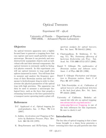
Optical TweezersOT - sjh,rd 3ABFF1zF2zFxx 12rayray 1CLaser beamFxray 2FzxzFigure 1: Ray model for the trapping force atthe focus of a laser beam. A particle displacedhorizontally (A) or vertically (B) from the focus(at x y z 0) refracts the light away fromthe focus, leading to a reaction force that pulls theparticle toward the focus; (C) Schematic of therestoring forces Fx and Fz versus displacement xand z of the particle from the trap center. Nearthe beam focus, Fx kx and Fz k 0 z.momentum. Momentum conservation impliesthat the scattered photon imparts an equaland opposite momentum change to the particle. The net force on the particle is a vectorequal and opposite the net rate of change ofmomentum of all the scattered laser photons.For particles with diameters d large compared to λ, the ray optics of reflection and refraction at the surface of the sphere provide agood model for the laser forces. The ray drawings in Figure 1 illustrate how laser beam refraction generates a trapping force. The laserbeam is directed in the positive z-directionand brought to a focus by a microscope objective. Note that, owing to wave diffraction,the focal region has nonzero width in the xydirection. Near the beam focus, a spherical dielectric particle alters the direction of a ray byrefracting it as shown in 1A. Momentum conservation implies that the particle experiencesa force, indicated by F in the figure, that is directed toward the beam focus. If the particleis located below the focus, it refracts the converging rays (such as rays 1 and 2) as shownin 1B. The corresponding reaction forces F1and F2 acting on the particle give a vectorsum F that is again directed toward the laserfocus. The net result of all the refractive scattering at any location in the vicinity of thefocus results in the gradient force that pullsthe particle into the beam focus. Reflectionat the boundaries between the sphere and themedium results in the scattering force in thedirection of the laser photons.For smaller particles of diameter d λ,Rayleigh scattering describes the interaction:The particle acts as a point dipole, scattering the incident beam in a spatially dependentfashion that depends on the particle’s locationin the laser field. The result is a net force Fgiven by d12 E (E B)(1)F α2dtwhere p αE gives the particle’s induceddipole moment. The first term is in the direction of the gradient of the field intensity, i.e.,the trapping force directed toward the laser focus. The second term gives the weaker scattering force—in the direction of the field’s Poynting vector E B.The center of the trap will be taken asr 0. For any small displacement (any direction) away from the trap center, the particle is subject to a Hooke’s law restoring force,i.e., proportional to and opposite the displacement. Detailed calculations show that theforce constant is sensitive to the shape andintensity of the laser field, the size and shapeOctober 14, 2020
OT - sjh,rd 4of the trapped particle, and the optical properties of the particle and surrounding fluid.Consequently, the Hooke’s law force is difficult to predict. Furthermore, our apparatusoperates in an intermediate regime of particlesizes where neither the ray optics nor Rayleighmodels are truly appropriate. The diameter dof the silica spheres (SiO2 ) range in size from0.5-5 µm. Thus with the laser wavelength ofλ 975 nm, we have d λ. Fortunately, wedo not need to calculate or predict the Hooke’slaw force constants based on these scatteringmodels. Instead, you will learn how to determine them in situ—from measurements madewith the particle in the trap.Consider the motion and forces in terms oftheir components. The laser beam in our apparatus is directed vertically upward, whichwill be taken as the z direction so that the xand y coordinates then describe the horizontal plane. Because the laser beam and focusing optics are cylindrically symmetric aroundthe z-axis, the trap has the same properties inthe x-direction as in the y-direction. We needonly consider the equations for the x motion ofthe particle, and a similar set of equations willdescribe the motion in the y-direction. However, the trapping force that acts along the zdirection is different than for x and y, as thelaser intensity in the focal region is clearly nota spherically symmetric pattern. The widthof the beam focus in its radial (xy) dimensionis very narrow. It is limited by wave diffraction to roughly one wavelength (λ 1µm),whereas this is not the case in z. Hence therestoring force in z is not necessarily as strongas in xy.If the focal “cone” has too shallow an angle(technically, a large f -number or small numerical aperture), particles may be trapped in thexy direction but not trapped along z. Thelaser beam will tend to pull small particles intoward the central optical axis and then pushOctober 14, 2020Advanced Physics Laboratorythem up and out of the trap. By employing alarge numerical aperture, our apparatus provides excellent trapping in all three directions.We will investigate the motions of the particle in the xy directions only. Consequently,in the discussion that follows, when forces, impulses, velocities or other vector quantities arewritten without vector notation (e.g., F instead of F) and without explicit directionalsubscripts (e.g., Fz k 0 z), they representthe x-component of the corresponding vectorquantity. For example, the trapping force inthe x-direction is simply Ftrap kx.What other forces act on the particle? Thelaser in our apparatus is directed verticallyupward—along the same axis as gravitationaland buoyant forces. Both silica spheres andbacteria are more dense than water and thusexperience a net downward force from thesesources. A constant force in the z-directionshifts the equilibrium position along the z-axisbut leaves the force constant unmodified. Forexample, the gravitational force on a mass mhanging from a mechanical spring of force constant k shifts the equilibrium by an amount mg/k, but the net force F kz stillholds with z now the displacement from thenew equilibrium point. Thus, the Fx kx,Fy ky, Fz k 0 z “trapping force” canand will be taken as relative to the final equilibrium position and includes not only thetrue trapping force centered at the laser focus, but also the laser scattering force andthe forces due to gravity and buoyancy. Keepin mind that these other forces are relativelyweak compared to the true trapping force andso the shift in the equilibrium position fromthe laser focus is rather small.The fluid environment supplies two additional and significant forces to the particle. The particles that we study with ourlaser tweezers are suspended in water wheremolecules are in constant thermal motion, i.e.,
Optical TweezersOT - sjh,rd 5they are moving with a range of speeds in random directions. For still water with no bulkflow, the x-component of velocity (or the component along any axis) is equally likely to bepositive as negative and will have an expectation value of zero: hvx i 0. Its mean squaredvalue is nonzero, however, as the average kinetic energy of the molecules is determinedby the temperature T . More precisely theequipartition theorem states that the meansquared value of any component of the velocity, e.g. hvx2 i, is related to the temperature Tby11m vx2 kB T(2)22where temperature is measured in Kelvin andkB 1.38 10 23 J/K is Boltzmann’s constant. The value of vx for any given particle isa random variable whose probability distribution is known as the Maxwell-Boltzmann distribution: vx21exp 2 dvxP (vx )dvx p2σv2πσv2(3)P (vx )dvx gives the probability that the velocity component vx for a given particle lies in therange between vx and vx dvx . The MaxwellBoltzmann distribution is a Gaussian distribution whose variance σv2 hvx2 i kB T /mmakes it satisfy the equipartition theorem.Likewise the other velocity components vy andvz obey the same distribution, (Eq. 3), withthe same variance σv2 .Exercise 1 (a) Find the root-mean-squarep(rms)velocityinthreedimensionh v 2 i qp vx2 vy2 vz23kB T /m for watermolecules near room temperature (23 C).(b) Find the rms x-component of velocity,phv 2 i σv and the number density of watermolecules (per unit volume). Use them to estimate the rate at which molecules cross through(in either direction) a 1 µm diameter disk oriented with its normal along the x-direction.Therefore, even if there is no bulk movementof the water, a small particle immersed in water is continuously subject to collisions frommoving water molecules. The collisional forceFi (t) exerted on the particle duringR the ithcollision delivers an impulse Ji Fi (t)dt tothe particle over the duration of the collision.By the impulse-momentum theorem, this impulse changes the particle momentum by thesame amount pi Ji ; impulse is momentumchange and they can be used somewhat interchangeably. For a one-micron particle in waterat room temperature, such collisions occur ata rate 1019 per second. Over some shorttime interval t, the total impulse p delivered to the particlePis the sum of the individualimpulses: p i Ji , and the average collisional force exerted on the particle over thisinterval is then Fc (t) p/ t.Theory cannot predict the individual impulses. A head-on collision with a high velocity water molecule delivers a large impulse,while a glancing collision with a low velocitymolecule delivers a smaller impulse. Depending on the direction of the collision, Ji canpoint in any direction. Even when summedover an interval t, p will include a randomcomponent.When no other forces act on the particle,the impulses push the particle slowly throughthe fluid along a random, irregular trajectory. This random motion is known as Brownian motion and is readily observed under amicroscope when any small (micron-sized orsmaller) particle is suspended in a fluid. Whenthe particle is trapped in an optical tweezers,the impulses continually push the particle inrandom directions. Because of the randomcomponent of the force, the particle motionis said to be stochastic (governed by probaOctober 14, 2020
OT - sjh,rd 6Advanced Physics Laboratorybility distributions), and only probabilities or force balance in order to relate the magnitudeaverage behavior can be predicted.of the microscopic impulses to the drag coefficient γ.Exercise 2 You can estimate the averageTherefore suppose that a micron-sized parspeed of Brownian motion from the fact that ticle is moving through a fluid. For claritythe speed of the microscopic particle at tem- we consider only one component (say x) of itsperature T must also satisfy the equipartition motion, although exactly the same argumentstheorem (2). For a silica sphere of diameter will apply to its motion in y and z. Let p1 µm and a density of 2.65 g/cm3 , what is its represent the x-component of the net vectorrms velocity at room temperature? Is your re- impulse p that is delivered to the particlesult still valid if the particle is in an optical during an interval t. Likewise v and p repretrap?sent the x-component of the velocity and momentum, and Ji is the x-component of impulseNote that if a particle moves through the from a single collision. Because of the high colfluid at a velocity v, collisions are not equally lision rate, t can be assumed short enoughlikely in all directions. More collisions will oc- that the particle velocity over this interval iscur on the side of the particle heading into effectively constant, but still long enough tothe fluid than on the trailing side and the to- allow, say, a few thousand collisions or more—tal impulse p that is acquired by the particle enough to apply the central limit theorem,will acquire a non-zero mean. The direction of which says that the sum p P pi will beithis impulse must tend to oppose the motion a random variable with a Gaussian probabilityof the particle through the fluid. Macroscop- distribution no matter what probability disically, we describe this effect by saying that tribution governs Ji . Moreover, the Gaussianthe particle experiences a viscous drag force distribution will have a mean µp h pi equalFdrag that is proportional to (and in opposite to the number of collisions times the mean ofdirection from) its velocitythe contributing Ji and it will have a varianceσp2 h( p µp )2 i equal to the number of colFdrag γv(4) lisionstimes the variance of the Ji . Becausethe number of collisions is proportional to t,where γ is the drag coefficient. As they haveboth the mean µp and the variance σp2 shouldthe same microscopic origin, there must bebe proportional to t.a connection between the magnitude of theThe total impulse p is therefore a randomsmall impulses p and the strength of thevariable that can be expressed asmacroscopic drag force. We can find this connection by noting that while the microscopic p µp δp(5)collisions deliver momentum to the particleand drive its Brownian motion, the overall where µp is a constant (associated with thedrag force tends to slow the particle down. On mean of the impulse distribution) and δp is aaverage these two effects must balance each zero-mean Gaussian random variable: hδpi other exactly, so that the particle neither slows 0 with a non-zero variance hδp2 i (associatedto a halt nor accelerates indefinitely. Rather with the variance of the impulse distribution).the particle maintains an average kinetic enIn a still fluid with no bulk flow, a partiergy in accord with the equipartition theorem cle at rest (v 0) experiences collisions from(Eq. 2). In the following we investigate this all directions equally. A collision delivering anOctober 14, 2020
Optical TweezersOT - sjh,rd 7impulse pi , is exactly as likely as a collisiondelivering pi . Consequently, p is equallylikely to be positive as negative and its expectation value is zero: µp 0. However if theparticle is moving through the fluid at velocity v, the impulses tend to oppose the motion(as discussed above) and we expect the average impulse µp will be proportional to v andopposite in sign. This tells us that the averagecollisional force µp / t is the x-component ofthe viscous drag force. Then from Eq. 4 wehaveµp γv(6) tHow does a Brownian particle slow down orspeed up due to µp and δp? How does this produce an average kinetic energy in agreementwith the equipartition theorem? The particle’s kinetic energy changes because the finalmomentum pf p p p µp δp differs from the initial momentum p mv. Theenergy change is given byp2fp2 i2m 2m 1 (p µp δp)2 p22m1µ2 δp2 2pδp 2m p 2µp p 2µp δp E (7)This energy change can be non-zero overany interval t; the particle can gain or loseenergy in the short term. However, if theparticle is to remain in thermal equilibriumover the long term, the average energy changeshould be zero. Applying the equilibrium condition h Ei 0 will allow us to relate thevariance of δp to factors associated with µp .Therefore we need to evaluate the expectationvalue of the right side of this expression, whichis simply the sum of the expectation values ofeach term:h Ei 1 2µp δp2 2 hpδpi2m 2 hµp pi 2 hµp δpi(8)Note first of all that the third term on theright side is 2 hpδpi 2m hvδpi. Because theparticle velocity v and the random part ofthe collisional impulse δp are statistically independent, the expectation value of their product is the product of their expectation values:hvδpi hvi hδpi. This term is zero because δpis a zero-mean random variable. The same applies to the last term in the parentheses, whichcontains the product 2 hµp δpi. Because δp israndom and uncorrelated with µp , this termwill also be zero.The first term on the right side involves µ2p ,where we have already noted that µp is proportional to the time interval t. Therefore thisis the only term in the expression that variesas t2 , while every other term is proportionalto t. Since we can choose t as small as welike, we can make this term arbitrarily small incomparison to the other terms. We can safelydiscard this term as an insignificant contribution to h Ei.Now we can use Eq. 6 relating the viscousdrag behavior and µp . Making the substitution µp γv t, we have the expectationvalue of the fourth term in Eq. 8: 2 hµp pi 2γ t hvpi 2mγ t hv 2 i. This term andthe remaining hδp2 i term then givehδp2 i2mkB Thδp2 i γ t (9)m2mwhere in the last line we used the equipartitiontheorem applied to the particle’s mean squarevelocity: hv 2 i kB T /m.Setting h Ei 0 and solving for hδp2 i thengivesδp2 2γkB T t(10)h Ei γ v 2 t October 14, 2020
OT - sjh,rd 8Advanced Physics LaboratoryNote this agrees with the prior assertion thathδp2 i should be proportional to t. Moreoverit gives the proportionality constant, 2γkB T ,that is needed to keep the velocity distribution in agreement with the equipartition theorem. Although derived for a particle movingalong the x-axis, this same expression will apply to each of the three dimensions, and so wefind the desired connection between the viscous drag coefficient, the mean squared random impulse (along any axis), and the temperature (i.e., the thermal equilibrium condition).Equation 10 leads directly to a versionof the fluctuation-dissipation theorem, whichsays that the variance of the fluctuating forcemust be proportional to the dissipative dragcoefficient γ and kB T . To see this, write thetotal collisional force as p tµpδp t t Fdrag (t) F (t)Fc (t) (11)where F (t) δp/ t and, since δp is a zeromean Gaussian random variable with a variance given by Eq. 10, F (t) will be a zero-meanGaussian random variable with a varianceF 2 (t) 2γkB T t(12)F (t) is called the Brownian force. In equilibrium, and on average, the energy lost by theparticle to the fluid via the drag force Fdrag (t)is balanced by the energy gained by the particle from the fluid via the fluctuating Brownianforce F (t).Note that different values of δp over anynon-overlapping time intervals arise from a different set of collisions and thus will be statistically independent. For example, even for adjacent time intervals, the two δp values wouldOctober 14, 2020be equally likely plus as minus. This independence implies F (t) is uncorrelated in timewith hF (t)F (t0 )i 0, for t 6 t0 (or, at least,for t t0 t). Thus, F (t) is a very oddforce that fluctuates virtually instantaneouslyon all but the shortest time scales.The local environment may produce otherforces on a small particle. The silica particlesin our experiment can adhere to a glass coverslip. A vesicle in a plant cell may be pulledthrough the cell by a molecular motor, while aswimming bacterium generates its own propulsion force by spinning its flagella. These additional forces compete with the trapping andfluid forces. If these forces are known, measurements of the displacements they cause canbe used to determine the strength of the trap.If the trap strength is known, measured displacements can be used to determine these additional forces. Subsequent sections describehow to use the physics of Brownian motionand viscous drag to determine the strength ofthe trapping and drag forces.We will need to know the position x of theparticle with respect to the trap. In principlewe could calculate x by analyzing microscopeimages collected with a camera. In practicethis does not work well because the displacements are very small and fluctuate rapidly.We can obtain higher precision and faster timeresolution if we detect the particle’s displacement indirectly by measuring the laser lightthat the particle deflects from the beam focus. Light scattered by the particle travelsdownstream (along the laser beam axis) and—in our apparatus—is measured on a quadrantphotodiode detector (QPD). The QPD is discussed in the experimental section. Here wemerely note that as the particle moves withinthe trap in either the x or x-direction, itdeflects some of the laser light in the same direction and the QPD reports this deflection bygenerating a positive or negative voltage V .
Optical TweezersOT - sjh,rd 9For small displacements x of the particlefrom the beam focus, the QPD voltage is linearin the displacement (V x). Consequently,we can writeV βx(13)We will refer to β (units of volts/meter) asthe detector constant. Because the voltagegenerated by the QPD depends on the totalamount of scattered light, β depends on thelaser power as well as the shape and size ofthe particle and other optical properties of theparticle and liquid.Analysis of Trapped MotionHow can we measure the strength of the trap?Suppose that a particle, suspended in water,is held in the optical trap. If we move themicroscope stage (that holds the sample slide)in the x direction at a velocity ẋdrive , the water(sealed in the slide) will move at that samevelocity. The water moves with the slide anddoes not slosh around because it is confined ina thin channel and experiences strong viscousforces with the channel walls. On the otherhand, the trap (whose position is determinedby the beam optics) will remain fixed so thatthe fluid and the trapped particle will then bein relative motion. The drag force is oppositethe relative velocity and thus given by γ(ẋ ẋdrive ). Like the Brownian force, the viscousforce is well-characterized and together theywill serve as calibration forces for the trap asdescribed next.Together with the viscous force above, thetrapping force kx, and the Brownian forceF (t), Newton’s 2nd law then takes the formmẍ(t) F (t) kx γ(ẋ ẋdrive )(14)where m is the particle mass and x is its displacement with respect to the equilibrium position of the trap.Macroscopically the drag coefficient γ is related to the viscosity of the fluid and the sizeand shape of the moving particle. For a sphereof radius a, γ is given by the Einstein-Stokesformulaγ 6πηa(15)where η is the dynamic viscosity of the fluid.While this equation is accurate for a spherical particle in an idealized fluid flow environment, the damping force is influenced by proximity to surfaces (the microscope slide) and issensitive to temperature and fluid compositionthrough the viscosity η. Thus it is appropriateto determine γ experimentally and compare itwith the Stokes Einstein prediction. A complete calibration includes a determination ofthe trap stiffness k, the detector constant β,and the drag coefficient γ.We use the calibration method designed byTolic-Norrelykke, et al. The basic idea is todrive the stage back and forth sinusoidallywith a known amplitude and frequency andmeasure (via the QPD detector voltage V ) theparticle’s response to the three forces. Becausethe physics of heavily damped motion of a particle in a fluid are well understood, the frequency characteristics of V (t) will reveal theparameters k, β, γ with good precision.You are probably familiar with underdamped oscillators, for which the drag term γ ẋ in Newton’s law is small in comparisonto the acceleration (“inertial”) term mẍ. Forsuch oscillators the acceleration is largely determined by the other (nonviscous) forces acting on the particle. However, the drag coefficient γ in a fluid generally scales as the radius a of the particle, whereas the mass mscales with the particle’s volume, m a3 .Consequently, for sufficiently small particles(a µm), the inertial term is far smaller thanthe drag term, mẍ γ ẋ . Under such conditions, the oscillator is strongly over-dampedand (to an excellent approximation) we mayOctober 14, 2020
OT - sjh,rd 10Advanced Physics Laboratorydrop the inertial term from Eq. 14. The parti- Recognizing the right hand side as a derivacle velocity is then determined by the balance tive, we findbetween the viscous force and the other forcesx(t) xT (t) xresp (t)(18)acting on the particle. Physically this meansthat, if any force is applied to the particle, wherethe particle “instantly” (see Exercise 3 below)Zaccelerates to its terminal velocity in the di1 t0F (t0 )e2πfc (t t) dt0(19)xT (t) rection of the applied force. When we dropγ the mẍ term, the equation of motio
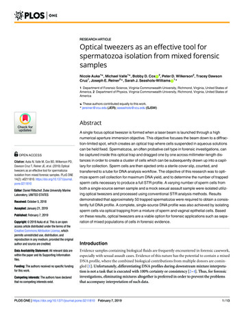
An optical tweezers apparatus uses a tightly focused laser to generate a trapping force that can capture and move small particles under a microscope. Because it can precisely and non-destructively manipulate objects such as indi-vidual cells and their internal components, the optical tweezers is extremely useful in biolog-ical physics research.