Transcription
Monaural Audio Source Separation using Variational AutoencodersLaxmi Pandey 1 , Anurendra Kumar 1 , Vinay Namboodiri11Indian Institute of Technology Kanpurlaxmip@iitk.ac.in, anu.ankesh@gmail.com, vinaypn@iitk.ac.inAbstractWe introduce a monaural audio source separation frameworkusing a latent generative model. Traditionally, discriminativetraining for source separation is proposed using deep neuralnetworks or non-negative matrix factorization. In this paper,we propose a principled generative approach using variationalautoencoders (VAE) for audio source separation. VAE computes efficient Bayesian inference which leads to a continuouslatent representation of the input data(spectrogram). It containsa probabilistic encoder which projects an input data to latentspace and a probabilistic decoder which projects data from latent space back to input space. This allows us to learn a robust latent representation of sources corrupted with noise andother sources. The latent representation is then fed to the decoder to yield the separated source. Both encoder and decoderare implemented via multilayer perceptron (MLP). In contrastto prevalent techniques, we argue that VAE is a more principled approach to source separation. Experimentally, we findthat the proposed framework yields reasonable improvementswhen compared to baseline methods available in the literaturei.e. DNN and RNN with different masking functions and autoencoders. We show that our method performs better than bestof the relevant methods with 2 dB improvement in the sourceto distortion ratio.Index Terms - Autoencoder, Variational inference, Latent variable, Source separation, Generative models, Deep learning*1. IntroductionThe objective of Monaural Audio Source Separation (MASS)is to extract independent audio sources from an audio mixturein a single channel. Source separation is a classic problem andhas wide applications in automatic speech recognition, biomedical imaging, and music editing. The problem is very challenging since it’s an ill-posed problem i.e. there can be manycombinations of solutions and the objective is to estimate thebest possible solution. Traditionally, the problem has been welladdressed by non-negative matrix factorization(NMF) [1] andPLCA[2] . These models learn the latent bases which are specific to a source from clean training data. These latent bases arelater utilized for separating source from the mixture signal [3].NMF and PLCA are generative models which work under theassumption that the data can be represented as the linear composition of low-rank latent bases. Several extensions of NMFand LVM have been employed in literature along with temporal, sparseness constraints [4, 1, 5]. Though NMF and PLCA arescalable, these techniques do not learn discriminative bases andtherefore yield worse results when compared to models where* Thefirst two authors contributed equallybases are learned on mixtures. Discriminative NMF [6] hasbeen proposed in order to learn mixture specific bases which inturn has shown some improvement over the NMF. NMF basedapproaches assume that data is a linear combination of latentbases and it may be a limiting factor for real-world data. Tomodel the non-linearity, deep neural networks(DNN), in various different configurations have been used in source separation[7, 8, 9]. The denoising auto-encoder (DAE) is a special typeof fully connected feedforward neural networks which can efficiently de-noise a signal [10]. They are used to learn robust lowdimensional features even when the inputs are perturbed withsome noise [11] . DAEs have been used for source separationwith input as a mixed signal and the output as the target source,both in form of spectral frames [12]. Though DAEs have a lotof advantages, it comes with the cost of high complexity and theloss in spatial information. Fully connected DAEs cannot capture the 2D (spectral-temporal) structures of the spectrogram ofthe input and output signals and have a lot of parameters to beoptimized and hence the system is highly complex. The fullyconvolutional denoising autoencoders [13] maps the distortedspeech signal to its clean speech signal with an application tospeech enhancement. Recently, a deep (stacked) fully convolutional DAEs (CDAEs) is used for the audio single channelsource separation (SCSS) [14]. However, current deep learningapproaches for source separation are still computationally expensive with a lot of parameters to tune and not scalable. NMFbased approaches, on the other hand, work with the simplisticassumption of linearity and the inability to learn discriminativebases effectively.In this paper, our goal is to have best of both worlds - i)To learn a set of bases effectively (which is done by encoderand decoder in VAE) and ii) Inexpensive computation. Moreover, unlike other methods, VAE can also yield the confidencescores of how good or bad are the separated sources, based onthe average posterior variance estimates. VAE has shown stateof-the-art in image generation, text generation and reinforcement learning [15, 16, 17, 18, 19]. In this paper, we show theeffectiveness of VAE for audio source separation. We comparethe performance of VAE with DNN/RNN architectures and autoencoders. VAE performs better than all methods in terms of asource to distortion ratio (SDR) with 2 dB improvement.2. Variational AutoencoderThe variational autoencoder [15] is a generative model whichassumes that an observed variable x is generated from an underlying random process with latent variable z as random variables.In this paper, we aim to learn a robust latent representation of anoisy signal i.e. P (z x) P (z x n), where x and n denotessignal and noise respectively. While estimating z for a source,we consider other sources as noise. The latent variable z is further used to estimate the clean (separated) source. Fig. 1 showsthe graphical model of VAE.
zxTFigure 1: Graphical model of VAE. T is total number of spectral frames. Dotted line denotes the inference of latent variablewhile solid line denotes the generative model of observed variable.Mathematically, the model can be represented as:Pθ (x, z) Pθ (x z)Pθ (z)ZPθ (x) Pθ (x z)Pθ (z)dz(1)(2)VAE assumes that the likelihood function Pθ (x z) and priordistribution Pθ (z) come from a parametric family of distributions with parameters θ. The prior distribution is assumed to bea Gaussian with zero mean and unit variance:P (z) N (z; 0, I)Pθ (x z) N (x; µθ (z), σθ2 (z)I)The audio single channel source separation (SCSS) aims to estimate the sources si (t), i from a mixed signal y(t) made up ofPI sources, y(t) Ii 1 si (t). We perform computations in theshort time Fourier transform (STFT) domain. Given the STFTof the mixed signal y(t), the primary goal is to estimate theSTFT of each source ŝi (t) in the mixture. Each of the sourcesis modeled using a single VAE i.e. a specific encoder and decoder for each source is learned. Fig. 2 shows the architectureof VAE used.Target SourceInput SignalPθ (x z)P (z)Pθ (z x) RPθ (x, z)dzFrequencyFrequencyµ, σ2TimeTimef(4)where, µθ (z) and σθ2 (z) are non-linear functions of z whichis modeled using a neural network. The posterior distributionPθ (z x) can be written by Bayes’s formula,µ σZ(Encoder)g(Decoder)Z: N(0,I)Figure 2: Architecture of VAE for audio source separation(5)However, the denominator is often intractable. Sampling methods like MCMC can be employed, but these are often too slowand computationally expensive. Variational Bayesian methods solves this problem by approximating the intractable trueposterior Pθ (z x) with some tractable parametric distributionqφ (z x). The marginal likelihood can be written as [15]log Pθ (x) DKL [qφ (z x) Pθ (z x)] L(θ, φ; x)(6)where,L(θ, φ; x) Eqφ (z x) [log Pθ (x, z) log qφ (z x)](7)where, E and DKL denotes the expectation and KL divergence respectively. The above marginal likelihood is againintractable due to KL divergence between approximate andtrue posterior, since we don’t know true distribution. Since,DKL 0, L(θ, φ; x) is called as (variational) lower boundand act as a surrogate for optimizing the marginal likelihood.Re-parameterizing the random variable z and optimizing withrespect to θ and φ yields [15],LXθ, φ argmax L(θ, φ : x) argmaxlog Pθ (x z l )θ,φ3. Source Separation(3)The likelihood, is often modeled using an independent Gaussiandistribution whose parameters are dependent on z,θ,φwhere, θ and φ are the parameters of multi layered perceptrons(MLP) for encoders and decoders respectively, L denotes thetotal number of samples used in sampling. Often a single sample is enough for learning θ and φ, if we have enough trainingdata [15]. Encoders and decoders are implemented via MLPnetworks with parameters θ and φ respectively. Normally, onelayer neural network is used for encoders and decoder in VAE.However, number of layers can be increased for increasing thenon-linearity. We call these as deep-VAE in the paper and showthat deep-VAE performs better than VAE.We propose to use as many VAEs as the number of sourcesto be separated from the mixed signal. Each VAE deals withthe mixed signal as a combination of a target source and background noise. These VAEs are trained to estimate the corresponding target sources from other background sources existingin the mixed signal. While training, VAEs map the magnitudespectrogram of the mixture to the magnitude spectrogram ofthe corresponding target sources. The inputs and outputs of theVAEs are 2D-segments from the magnitude spectrograms of themixed and target signals respectively. This facilitates the VAEscapability to capture the time-frequency characteristics of eachsource by spanning multiple time frames.3.0.1. Training and Testing of VAEs for Source SeparationLet’s assume that we have training data as mixed signals andtheir corresponding clean sources. Let Ytr be the magnitudespectrogram of the mixed signal and Si be the magnitude spectrogram of the clean source i. The VAE of source i is trained tomaximize the following likelihood function :θ, φ argmaxθ,φLXlog Pθ (Si z l ) DKL [qφ (z l Ytr ) P (z)]l 1l 1 DKL [qφ (z l x) P (z)]Code and data: github.com/anurendra/vae sep(8)In practice, L 1 in our set up leads to good learning ofencoder and decoder. Given the trained VAEs, the magnitudespectrogram Y of the mixed signal is passed through all the
Figure 3: Performance comparison of VAE ([513 128 64]) and deep VAE ([513 256 192 128 64]) with the baseline i.e. DNN and RNNwith different masking function [7] and autoencoders [14].88866642To validate the performance of the proposed model, we performspeaker source separation experiments on the TIMIT database[20]. To obtain the spectrogram from an audio signal, we perform short term Fourier transform (STFT) with 64 ms windowand 16 ms overlap. Only magnitude of spectrogram were givenas input to the algorithm. Finally, the separated time-domainspeech was obtained by multiplying phase of the mixed signal with the magnitude of the separated spectrogram [2]. Wehave used a total of ten speakers (5 male and 5 female) fromthe database which includes speech data for five male and fivefemale speakers sampled at 16 KHz. We normalize each ofthe signals to zero mean and unit variance. The training mixtures are obtained by linear addition of each male and femaleaudio signals resulting in 25 mixtures at 0 dB signal to noiseratio (SNR). We trained five VAEs for five male and five female speakers respectively. The first 20 mixtures (4 for eachmale and female speaker) were used as input to VAE to train allnetworks for separation, and the last 5 mixtures were used fortesting. For the input and output data for the VAEs, only magnitude of spectrogram was given as input to the encoder. Wechose 17 frames as the number of spectral frames in each 2Dsegment. So, the dimension of each input and output(target) foreach VAE is 17 (time frames) * 513 (frequency bins). Finally,the separated time-domain speech was obtained by multiplyingphase of the mixed signal with the magnitude of the separatedspectrogram.We use perceptually motivated scores as measure of evaluation and subsequently use BSS-EVAL TOOLBOX [21]. It proposes three metrics namely i) Source to distortion ratio (SDR)ii) Source to interference ratio (SIR) and iii) Source to artifactratio (SAR).4.2. Parameter SelectionThe parameters of VAE were selected based on source separation results as evaluated on perceptual metrics described above.4204.1. Experimental DetailsdBIn this section, we describe the experiments done for parameterselection of the model and it’s comparative advantage over otherexisting deep learning architectures. We do parameter selectionfor latent dimension (K), batch size and encoder and decoderdimensions in VAE and deep VAE. We finally do the performance comparison of speaker source separation and show thatVAE performs better or comparative to baseline methods.We fixed all the dimensions except that of latent dimension K,which was varied in [16 32 64 128 256 512]. The middle layerin encoder and decoder was fixed as 128, which was separatelytuned.dB4. Experiments4.2.1. Number of latent dimension(K)dBtrained VAEs. The output of the VAE of source i is the estimateof the spectrogram S̃i of source i.500Latent Dimension(a) SDR420500Latent Dimension(b) SIR0500Latent Dimension(c) SARFigure 4: Performance comparison for different latent spacedimension [16 32 64 128 256 512]Fig. 4 shows the plot of source separation for a speakerin terms of SDR, SIR and SAR for different values of K. Wesee that model performs best for all the metrics when K 64.Therefore we fix the latent dimension as 64 in later experiments.4.2.2. Batch sizeThe magnitude spectrogram has temporal dependency along thedirection of time. VAE learns the existing spatio-temporal structure from each batch of the spectrogram. There is a trade-offbetween increasing and decreasing batch size. As batch-sizeincreases, VAE is able to extract long-term temporal featuresefficiently. However, it leads to loss of time specific structures.Also, lesser training data leads to a worse estimate of encoderand decoder. Very small batch size, on the other hand, does notallow VAE to learn the long-term temporal dependencies. Table1 shows the performance of source separation as batch size isvaried. Based on the results in the table, we fix batch size to be17 in the rest of the experiments.Table 1: Performance of proposed framework for different batchsize in terms of SDR, SIR and SAR.Batch size11017305070Evaluation MetricsSDR SIR 71.162.667.026.956.927.11
Table 2: Performance of deep-VAE in terms of SDR, SIR andSAR.# Encoder Layers[513 64][513 128 64][513 256 128 64][513 256 192 128 64]Evaluation MetricsSDR SIR 84.3. Confidence ScoreUnlike other existing source separation methods, VAE alsoyields posterior variance estimates of the separated sources. Wecalculate the average posterior variance as a proxy for the confidence scores of how good or bad are the separated sources. Alower variance implies that the distribution is peaky at mean andthe confidence score is high. As discussed earlier, the signal tonoise ratio for training data is (0 dB). For test signals, we varythe signal to noise ratio (SNR) and compute the average posterior variance. Fig. 5 shows the average posterior variance asSNR varies. It can be observed that average variance decreasesas SNR increases (except at 0 dB). The anomaly at 0 dB canbe attributed to the fact that VAE was trained on 0 dB SNR.Fig. 6 shows the reconstructed spectrogram in the case of different signal to noise ratios. We observe that the reconstructionspectrogram becomes noisy as SNR decreases.Average Posterior Variance5Frequency4000Frequency4000FrequencyThe success of VAE lies in it’s ability to learn the non-linearcombination, and yet able to learn the posterior distributionsefficiently. Therefore, we hypothesize that increasing numberof layers in deep-VAE should yield better source separation.We use rectified linear units (ReLU) as the non-linearity everywhere in our network. We vary the number of layers keeping thelatent dimension fixed to 64, found earlier. Table 2 shows theresults. We see that the performance increases as the numberof layer increases. However, deep architectures doesn’t yield asubstantial improvement given that these come at the cost of being more computationally expensive. The preference of DeepVAE over VAE would, therefore, be dependent on the trade-offbetween accuracy and computational availability.4000Frequency4.2.3. Number of 0.511.52(d)TimeFigure 6: (a): Target source (b): Reconstructed signal (SNR 4.7 dB) (c): Reconstructed signal (SNR 0 dB) (d): Reconstructed signal (SNR -0.69 dB)all evaluation metrics with 3 dB improvement in SDR, 2dB in SIR and 0.5 dB in SAR. Fig. 3 shows performancecomparison of VAE and deep-VAE with baseline approaches.We see that VAE and deep-VAE perform best in terms of SDRwith 2 dB improvement. In terms of SIR, Binary-mask approach performs the best. However, both VAE and deep-VAEprovide good results in terms of all three measures. Note thatfor source separation, SDR would be considered the more important evaluation measure in which Binary-mask method performs far lower. While SDR captures overall noise, SIR andSAR captures only interference and artifact noise respectively[21]. This implies that VAE is able to remove noise (measured by SDR) better than all other models by capturing thespatio-temporal characteristic of spectrogram in latent space effectively. We also observe that SAR in VAE and deep-VAE isbetter than existing approaches. This shows that artifact introduced by VAE and deep VAE (measured by SAR) is lesser thanother models.Table 3: Performance of proposed method in terms of SDR, SIRand SAR.MethodsVAE3Deep FemaleMaleFemaleMaleFemaleEvaluation MetricsSDR SIR 66.116.527.276.777.386.9821.5-2024SNR (dB)Figure 5: Variation of average posterior variance with SNR4.4. Performance AnalysisWe do perform analysis of VAE for source separation by comparing our algorithm with baseline approaches. We compare theperformance of source separation with the existing deep learning approaches [7, 8] and autoencoders using a number of evaluation metrics. Table 3 shows the performance comparison ofsource separation of male and female individually with autoencoders. We see that VAE and deep-VAE performs better on5. ConclusionsIn this work, we proposed a variational autoencoder basedframework for monaural audio source separation. We showedthat VAE is able to learn the inherent latent representation of asource by encoding the non-linear dependencies. The performance of the proposed framework is evaluated on audio sourceseparation. The proposed framework yields reasonable improvements when compared to baseline methods. However, theframework requires prior knowledge of the sources in the mixture and a corresponding VAE has to be used (which alloweddiscriminative ability). Future works will be directed towardsdeveloping a single VAE for many/similar sources.
6. References[1] T. Virtanen, “Monaural sound source separation by nonnegativematrix factorization with temporal continuity and sparseness criteria,” IEEE transactions on audio, speech, and language processing, vol. 15, no. 3, pp. 1066–1074, 2007.[2] P. Smaragdis, B. Raj, and M. Shashanka, “A probabilistic latentvariable model for acoustic modeling,” NIPS, vol. 148, pp. 8–1,2006.[3] B. Raj, M. V. Shashanka, and P. Smaragdia, “Latent dirichlet decomposition for single channel speaker separation,” in ICASSP,vol. 5. IEEE, 2006.[4] N. Mohammadiha, P. Smaragdis, G. Panahandeh, and S. Doclo,“A state-space approach to dynamic nonnegative matrix factorization,” IEEE Transactions on Signal Processing, vol. 63, no. 4, pp.949–959, 2015.[5] P. Smaragdis, C. Fevotte, G. J. Mysore, N. Mohammadiha, andM. Hoffman, “Static and dynamic source separation using nonnegative factorizations: A unified view,” IEEE Signal ProcessingMagazine, vol. 31, no. 3, pp. 66–75, 2014.[6] F. Weninger, J. Le Roux, J. R. Hershey, and S. Watanabe, “Discriminative nmf and its application to single-channel source separation.” in INTERSPEECH, 2014, pp. 865–869.[7] P.-S. Huang, M. Kim, M. Hasegawa-Johnson, and P. Smaragdis,“Deep learning for monaural speech separation,” in Acoustics,Speech and Signal Processing (ICASSP), 2014 IEEE International Conference on. IEEE, 2014, pp. 1562–1566.[8] ——, “Joint optimization of masks and deep recurrent neural networks for monaural source separation,” IEEE/ACM Transactionson Audio, Speech and Language Processing (TASLP), vol. 23,no. 12, pp. 2136–2147, 2015.[9] A. A. Nugraha, A. Liutkus, and E. Vincent, “Multichannel audiosource separation with deep neural networks,” IEEE/ACM Transactions on Audio, Speech, and Language Processing, vol. 24,no. 9, pp. 1652–1664, 2016.[10] X. Lu, Y. Tsao, S. Matsuda, and C. Hori, “Speech enhancementbased on deep denoising autoencoder.” in Interspeech, 2013, pp.436–440.[11] P. Vincent, H. Larochelle, Y. Bengio, and P.-A. Manzagol, “Extracting and composing robust features with denoising autoencoders,” in Proceedings of the 25th international conference onMachine learning. ACM, 2008, pp. 1096–1103.[12] M. Kim and P. Smaragdis, “Adaptive denoising autoencoders: Afine-tuning scheme to learn from test mixtures,” in InternationalConference on Latent Variable Analysis and Signal Separation.Springer, 2015, pp. 100–107.[13] S. R. Park and J. Lee, “A fully convolutional neural network forspeech enhancement,” arXiv preprint arXiv:1609.07132, 2016.[14] E. M. Grais and M. D. Plumbley, “Single channel audio sourceseparation using convolutional denoising autoencoders,” arXivpreprint arXiv:1703.08019, 2017.[15] D. P. Kingma and M. Welling, “Auto-encoding variational bayes,”arXiv preprint arXiv:1312.6114, 2013.[16] D. J. Rezende, S. Mohamed, and D. Wierstra, “Stochastic backpropagation and approximate inference in deep generative models,” arXiv preprint arXiv:1401.4082, 2014.[17] K. Gregor, I. Danihelka, A. Graves, D. J. Rezende, and D. Wierstra, “Draw: A recurrent neural network for image generation,”arXiv preprint arXiv:1502.04623, 2015.[18] C. Doersch, “Tutorial on variational autoencoders,” arXiv preprintarXiv:1606.05908, 2016.[19] U. Jain, Z. Zhang, and A. Schwing, “Creativity: Generating diverse questions using variational autoencoders,” arXiv preprintarXiv:1704.03493, 2017.[20] J. S. Garofolo, L. F. Lamel, W. M. Fisher, J. G. Fiscus, and D. S.Pallett, “Darpa timit acoustic-phonetic continous speech corpuscd-rom. nist speech disc 1-1.1,” NASA STI/Recon technical reportn, vol. 93, 1993.[21] C. Févotte, R. Gribonval, and E. Vincent, “Bss eval toolbox userguide–revision 2.0,” 2005.
their corresponding clean sources. Let Y tr be the magnitude spectrogram of the mixed signal and S ibe the magnitude spec-trogram of the clean source i. The VAE of source iis trained to maximize the following likelihood function : ; argmax ; XL l 1 log P (S i j z l) D KL[q Y tr)jj )] In practice, L 1 in our set up leads to good .