Transcription
A Tutorial OnBackward Propagation Through Time (BPTT)In The Gated Recurrent Unit (GRU) RNNMinchen LiDepartment of Computer ScienceThe University of British Columbiaminchenl@cs.ubc.caAbstractIn this tutorial, we provide a thorough explanation on how BPTT in GRU1 isconducted. A MATLAB program which implements the entire BPTT for GRUand the psudo-codes describing the algorithms explicitly will be presented. Weprovide two algorithms for BPTT, a direct but quadratic time algorithm for easyunderstanding, and an optimized linear time algorithm. This tutorial starts witha specification of the problem followed by a mathematical derivation before thecomputational solutions.1SpecificationWe want to use a dataset containing ns sentences each with nw words to train a GRU languagemodel, and our vocabulary size is nv . Namely, we have input x Rnv nw ns and label y Rnv nw ns both representing ns sentences.For simplicity, lets look at one sentence at a time. In one sentence, the one-hot vector xt Rnv 1represents the tth word. For time step t, the GRU unit computes the output ŷt using the input xt andthe previous internal state st 1 as follows:ztrthtstŷt σ(Uz xt Wz st 1 bz ) σ(Ur xt Wr st 1 br ) tanh(Uh xt Wh (st 1 rt ) bh ) (1 zt ) ht zt st 1 sof tmax(V st bV )(1)Here is the vector element-wise multiplication, σ() is the element-wise sigmoid function, andtanh() is the element-wise hyperbolictangent function. The dimensions of the parameters are asfollows:Uz , Ur , Uh Rni nvWz , Wr , Wh Rni nibz , br , bh Rni 1V Rnv ni , bV Rnv 1where ni is the internal memory size set by the user.1GRU is an improved version of traditional RNN (Recurrent Neural Network, see WildML.com for an introduction. This link also provides an introduction to GRU and some general discussion on BPTT and beyond.)
Then for step t, we can calculate the cross entropy loss Lt as: Lt sumOf AllElements yt log(ŷt )(2)Here log is also an element-wise function.To train the GRU, we want to know the values of all parameters that minimize the total loss L Pnwt 1 Lt :argmin LΘwhere Θ {Uz , Ur , Uc , Wz , Wr , Wc , bz , br , bc , V, bV }. This is a non-convex problem with hugeinput data. So people usually use Stochastic Gradient Descent2 method to solve this problem, whichmeans we need to calculate L/ Uz , L/ Ur , L/ Uh , L/ Wz , L/ Wr , L/ Wh , L/ bz , L/ br , L/ bh , L/ V , L/ bV given a batch of sentences. (Note that in each step, theseparameters stays the same.) In this tutorial we consider using only one sentence at a time to make itconcise.2DerivationThe best way to calculate gradients using the Chain Rule from output to input is to first draw theexpression graph of the entire model in order to figure out the relations between the output, intermediate results, and the input3 . Here we draw part of the expression graph of GRU in Fig.1.Figure 1: The upper part of expression graph describing the operations of GRU. Note that the subgraph which st 1 depends on is just like the sub-graph of st . This is what the red dashed linesmean.With this expression graph, the Chain Rule works if you go backwards along the edges (top-down).If a node X has multiple outgoing edges connecting the target node T , you need to sum over thepartial derivatives of each of those outgoing edges to derive the gradient T / X. We will illustratethe rules in the following paragraphs.PnwLet’s take L/ Uz as the example here. Others are just similar.t 1 Lt and thePnwSince L parameters stay the same in each step, we also have L/ Uz t 1 ( Lt / Uz ), so let’s calculateeach Lt / Uz independently and sum them up.23See the Wikipedia to get some knowledge about Stochastic Gradient Descent.See colah’s blog and Stanford CS231n Course Note for some general introductions.2
With the Chain Rule, we have: Lt Lt st(3) Uz st UzThe first part is just trivial if you know how to differentiate the cross entropy loss function embeddedwith the sof tmax function: Lt V (ŷt yt ) stFor z/ Uz , similarly, some people might just derive: (if they know how to differentiate sigmoidfunction) st (st 1 ht ) zt (1 zt ) xTt(4) UzHere there are two expressions 1 z and z st 1 influencing st / z as shown in our expressiongraph. The solution is to derive partial derivatives through each edge and then add them up, whichis exactly how we deal with st / st 1 as you will see in the following paragraphs. However, Eq.4only calculates one part of the gradient, so we put a bar on top of it, while you may find this veryuseful in our following calculations.Note that st 1 also depends on Uz , so we can not treat it as a constant here. Moreover, this st 1will also introduce the influence of si , where i 1, ., t 2. So for clearness, we should expandEq.3 as: Lt Lt st Uz st Uzt Lt X st si (5) st si Uzi 1tt 1 Lt X Y sj 1 si st i 1 sj Uzj iwhere si / Uz is the gradient of si with respect to Uz while taking si 1 as a constant, of which asimilar example has been shown in Eq.4 for step t.The derivation of st / st 1 is similar to the derivation of st / z as has been discussed above.Since there are four outgoing edges from st 1 to st directly and indirectly through zt , rt , and ht inthe expression graph, we need to sum all the four partial derivatives together: st st ht st zt st st 1 ht st 1 zt st 1 st 1 st ht rt ht st zt st ht rt st 1 st 1 zt st 1 st 1(6)where st / st 1 is the gradient of st with respect to st 1 while taking ht and zt as constants.Similarly, ht / st 1 is the gradient of ht with respect to st 1 while taking rt as a constant.Plugging the intermediate results in the above formula, we get: st (1 zt ) WrT ((WhT (1 h h)) st 1 r (1 r)) ((WhT (1 h st 1 WzT (st 1 ht ) zt (1 zt ) zh)) rt Till now, we have covered all the components needed to calculate Lt / Uz . The gradient of Lt withrespect to other parameters are just similar. In the next chapter, we will provide a more machineryview of the calculation - the psudo-code describing the algorithm to calculate the gradients. In thelast chapter of this tutorial, we will provide the pure machine representation - a MATLAB programwhich implements the calculation and verification of BPTT. If you just want to understand the ideabehind BPTT and decide to use fully supported auto-differentiation packages (like Theano4 ) to buildyour own GRU, you can stop here. If you need to implement the exact chain rule like us or justcurious about what will happen next, get ready to proceed!4Theano is a Python library that allows you to define, optimize, and evaluate mathematical expressionsinvolving multi-dimensional arrays efficiently.3
3AlgorithmHere we also only take L/ Uz as the example. We will provide the calculation of all the gradientsin the next chapter.We present two algorithms, one direct algorithm as derived previously calculating Lt / Uz andsum them up while taking O(n2w ) time, and the other O(nw ) time algorithm which we will see later.Algorithm 1 A direct but O(n2w ) time algorithm to calculate L/ Uz (and beyond)Input: The training data X, Y Rnv nw composed of the one-hot column vectors xt , yt Rnv 1 ,t 1, 2, ., nw representing the words in the sentence.Input: A vector s0 Rni 1 representing the initial internal state of the model (usually set to 0).Input: The parameters Θ {Uz , Ur , Uc , Wz , Wr , Wc , bz , br , bc , V, bV } of the model.Output: The total loss gradient L/ Uz .1: %forward propagate to calculate the internal states S Rni nw , the predictions Ŷ Rnv nw ,the losses Lmtr Rnw 1 , and the intermediate results Z, R, C Rni nw of each step:2: [S, Ŷ , Lmtr , Z, R, C] f orward(X, Y, Θ, s0 ) % forward() can be implemented easily according to Eq.1 and Eq.23: dUz zeros(ni , nv ) % initialize a variable dUz4: Lmtr / S V T (Ŷ Y ) % calculate Lt / st for t 1, 2, ., nw with one matrix operation5: for t 1 to nw % calculate each Lt / Uz and accumulate6:for j t to 1 % calculate each ( Lt / sj )( sj / Uz ) and accumulate7: Lt / zj Lt / sj (sj 1 hj ) % sj / zj is (sj 1 hj ), Lt / sj is calculatedin the last inner loop iteration or in Line 4 Lt / (Uz xj Wz sj 1 bz ) Lt / zj zj (1 zj ) % σ(x)/ x σ(x)σ(x)) 9:dUz Lt / (Uz xj Wz sj 1 bz ) xTj % accumulate8:(1 10:calculate Lt / sj 1 using Lt / sj and Eq.6 % for the next inner loop iteration11:end12: end13: return dUz % L/ UzThe above direct algorithm actually follows Eq.5 to calculate Lt / Uz and then add them up toform L/ Uz :nwX L Lt Uz Uzt 1 nw tX Lt X st si st i 1 si Uzt 1nw tt 1X Lt X Y sj 1 si t 1 sti 1j i sj UzIf we just expand Lt / Uz to the second line of the above equation and do some reordering, we canget:nw tX L Lt X st si Uz st i 1 si Uzt 1 nw Xt X Lt st si st si Uzt 1i 1nw Xt X Lt si si Uzt 1i 14
Right now the inner summation keeps the subscript of Lt and iterate over si . If we further expandthe inner summation and then sort them to iterate over Li , we get:nnw XwX Li st L Uz st Uzt 1i t(7)For the inner summation of Eq.7, we have:nw X Li i t st nw X Li st 1 Lt st 1 st sti t 1nw X(8) Lt Li st 1 s s stt 1ti t 1This just gives us an updating formula to calculate this inner summation for each step t incrementallyrather than executing another f or loop, thus making it possible for us to implement an O(nw ) timealgorithm!Algorithm 2 An optimized O(nw ) time algorithm to calculate L/ Uz (and beyond)Input: The training data X, Y Rnv nw composed of the one-hot column vectors xt , yt Rnv 1 ,t 1, 2, ., nw representing the words in the sentence.Input: A vector s0 Rni 1 representing the initial internal state of the model (usually set to 0).Input: The parameters Θ {Uz , Ur , Uc , Wz , Wr , Wc , bz , br , bc , V, bV } of the model.Output: The total loss gradient L/ Uz .1: %forward propagate to calculate the internal states S Rni nw , the predictions Ŷ Rnv nw ,the losses Lmtr Rnw 1 , and the intermediate results Z, R, C Rni nw of each step:2: [S, Ŷ , Lmtr , Z, R, C] f orward(X, Y, Θ, s0 ) % forward() can be implemented easily according to Eq.1 and Eq.23: dUz zeros(ni , nv ) % initialize a variable dUz4: Lmtr / S V T (Ŷ Y ) % calculatet 1, 2, ., nw with one matrix operation Lt / s t for 5: for t nw to 1 % calculate eachPnwPnwi t Li st st Uzand accumulate P nwi t ( Li / st )(st 1 ht ) % st / zt is (st 1 ht ),i t ( Li / zt ) Pnw( L/ s)iscalculatedinthelastiterationor in Line 4.(when t nw ,itPi tnw( L/ s) L/ s)ittti t P Pnwnw7:( L/ (Ux Wzt (1 zt ) % σ(x)/ x iz tz st 1 bz )) i ti t ( Li / zt )6:(1 σ(x)) PnwdUz ( L/ (Ux Ws b))xTt % accumulateiztzj tzi tPnwcalculate i t 1( Li / st 1 ) using Eq.6 and Eq.8 % for the next iterationendreturn dUz % L/ Uzσ(x)8:9:10:11:5
4ImplementationHere we provide the MATLAB program which calculates the gradients with respect to all the parameters of GRU using our two proposed algorithms. It also checks the gradients with the numericalresults. We will divide our code into two parts, the first part presented below contains the corefunctions implementing the BPTT of GRU we just derived, the second part is composed of somefunctions that are less important to the topic of this tutorial.Core Functions13%%%%This programWe c a l c u l a t ecompare themderivation ist e s t s t h e BPTT p r o c e s s we m a n u a l l y d e v e l o p e d f o r GRU.t h e g r a d i e n t s o f GRU p a r a m e t e r s w i t h c h a i n r u l e , and t h e nto t he numerical g r a d i e n t s to check whether our chain r u l ecorrect .579% Here , we p r o v i d e d 2 v e r s i o n s o f BPTT , b a c k w a r d% The f o r m e r one i s t h e d i r e c t i d e a t o c a l c u l a t estep% and add them up (O( s e n t e n c e s i z e ˆ 2 ) t i m e ) . Theto% c a l c u l a t e the c o n t r i b u t i o n of each s t e p to theis% o n l y O( s e n t e n c e s i z e ) t i m e .d i r e c t ( ) and b a c k w a r d ( ) .g r a d i e n t w i t h i n eachl a t t e r one i s o p t i m i z e do v e r a l l g r a d i e n t , which111315% T h i s i s v e r y h e l p f u l f o r p e o p l e who w a n t s t o i m p l e m e n t GRU i n C a f f esince% Caffe didn ’ t s u p p o r t auto d i f f e r e n t i a t i o n . This i s a l s o very h e l p f u lfor% t h e p e o p l e who w a n t s t o know t h e d e t a i l s a b o u t B a c k p r o p a g a t i o n Through% Time a l g o r i t h m i n t h e R e c c u r e n t N e u r a l N e t w o r k s ( s u c h a s GRU and LSTM)% and a l s o g e t a s e n s e on how a u t o d i f f e r e n t i a t i o n i s p o s s i b l e .171921%%%%NOTE : We d i d n ’ t i n v o l v e SGD t r a i n i n g h e r e . With SGD t r a i n i n g , t h i sp r o g r a m would become a c o m p l e t e i m p l e m e n t a t i o n o f GRU which c a n bet r a i n e d w i t h s e q u e n c e d a t a . However , s i n c e t h i s i s o n l y a CPU s e r i a lM a t l a b v e r s i o n o f GRU, a p p l y i n g i t on l a r g e d a t a s e t s w i l l bedramatically% slow .23% by Minchen Li , a t The U n i v e r s i t y o f B r i t i s h Columbia . 2016 04 21252729313335373941434547f u n c t i o n testBPTT GRU% s e t GRU and d a t a s c a l evocabulary size 64;iMem size 4;s e n t e n c e s i z e 2 0 ; % number o f words i n a s e n t e n c e%( i n c l u d i n g s t a r t and end symbol )% s i n c e we w i l l o n l y u s e one s e n t e n c e f o rtraining ,% t h i s is also the t o t a l steps during t r a i n i n g .[x y] getTrainingData ( vocabulary size , sentence size ) ;% i n i t i a l i z e parameters :% m u l t i p l i e r f or input x t of i n t e r m e d i a t e v a r i a b l e sU z r a n d ( iMem size , v o c a b u l a r y s i z e ) ;U r r a n d ( iMem size , v o c a b u l a r y s i z e ) ;U c r a n d ( iMem size , v o c a b u l a r y s i z e ) ;% m u l t i p l i e r f or pervious s of i n t e r m e d i a t e v a r i a b l e sW z r a n d ( iMem size , i M e m s i z e ) ;W r r a n d ( iMem size , i M e m s i z e ) ;W c r a n d ( iMem size , i M e m s i z e ) ;% bias terms of i n t e r m e d i a t e v a r i a b l e sb z r a n d ( iMem size , 1 ) ;6
bb%Vb%s495153r r a n d ( iMem size , 1 ) ;c r a n d ( iMem size , 1 ) ;decoder for generating output rand ( v o c a b u l a r y s i z e , iMem size ) ;V rand ( vocabulary size , 1) ; % bias of decoderprevious s of step 10 r a n d ( iMem size , 1 ) ;55% c a l c u l a t e and c h e c k g r a d i e n ttic[ dV , db V , dU z , dU r , dU c , dW z , dW r , dW c , db z , d b] .backward direct (x , y , U z , U r , U c , W z, W r , W c,, V, b V , s 0 ) ;tocticcheckGradient GRU ( x , y , U z , U r , U c , W z , W r , W c , bV, b V , s 0 , . . .dV , db V , dU z , dU r , dU c , dW z , dW r , dW c , db z ,ds 0 ) ;toc57596163r , db c , d s 0b z, b r , b cz, b r , b c,d b r , db c ,65tic[ dV , db V , dU z , dU r , dU] .backward ( x , y , U z , Ub V, s 0);tocticcheckGradient GRU ( x , y , UV, b V , s 0 , . . .dV , db V , dU z , dU r ,ds 0 ) ;toc67697173c , dW z , dW r , dW c , db z , d b r , db c , d s 0r , U c , W z , W r , W c , b z , b r , b c , V,z , U r , U c , W z, W r, W c, b z , b r , b c ,dU c , dW z , dW r , dW c , db z , d b r , db c ,end75777981838587899193959799101% F o r w a r d p r o p a g a t e c a l c u l a t e s , y h a t , l o s s and i n t e r m e d i a t e v a r i a b l e sf o r each s t e pfunction [ s , y hat , L , z , r , c ] forward (x , y , . . .U z , U r , U c , W z , W r , W c , b z , b r , b c , V, b V , s 0 )% count s i z e s[ vocabulary size , sentence size ] size (x) ;i M e m s i z e s i z e (V, 2 ) ;%syLzrcinitialize results z e r o s ( iMem size , s e n t e n c ehat zeros ( vocabulary size , zeros ( s e n t e n c e s i z e , 1) ; z e r o s ( iMem size , s e n t e n c e z e r o s ( iMem size , s e n t e n c e z e r o s ( iMem size , s e n t e n c esize ) ;sentence size ) ;size ) ;size ) ;size ) ;% c a l c u l a t e r e s u l t for step 1 since s 0 i s not in sz ( : , 1 ) s i g m o i d ( U z x ( : , 1 ) W z s 0 b z ) ;r ( : , 1 ) s i g m o i d ( U r x ( : , 1 ) W r s 0 b r ) ;c ( : , 1 ) t a n h ( U c x ( : , 1 ) W c ( s 0 . r ( : , 1 ) ) b c ) ;s ( : , 1 ) (1 z ( : , 1 ) ) . c ( : , 1 ) z ( : , 1 ) . s 0 ;y h a t ( : , 1 ) s o f t m a x (V s ( : , 1 ) b V ) ;L ( 1 ) sum( y ( : , 1 ) . l o g ( y h a t ( : , 1 ) ) ) ;% calculate results for step 2 sentence size similarlyf o r wordI 2 : s e n t e n c e s i z ez ( : , w o r d I ) s i g m o i d ( U z x ( : , w o r d I ) W z s ( : , wordI 1) b z ) ;r ( : , w o r d I ) s i g m o i d ( U r x ( : , w o r d I ) W r s ( : , wordI 1) b r ) ;c ( : , w o r d I ) t a n h ( U c x ( : , w o r d I ) W c ( s ( : , wordI 1) . r ( : , w o r d I ) ) b c);7
s ( : , w o r d I ) (1 z ( : , w o r d I ) ) . c ( : , w o r d I ) z ( : , w o r d I ) . s ( : , wordI103 1) ;y h a t ( : , w o r d I ) s o f t m a x (V s ( : , w o r d I ) b V ) ;L ( w o r d I ) sum( y ( : , w o r d I ) . l o g ( y h a t ( : , w o r d I ) ) ) ;105end107109111113115117119121123125end% Backward p r o p a g a t e t o c a l c u l a t e g r a d i e n t u s i n g c h a i n r u l e% (O( s e n t e n c e s i z e ) t i m e )f u n c t i o n [ dV , db V , dU z , dU r , dU c , dW z , dW r , dW c , db z , d b r , db c ,ds 0 ] . . .b a c k w a r d ( x , y , U z , U r , U c , W z , W r , W c , b z , b r , b c , V, b V ,s 0)% f o r w a r d p r o p a g a t e t o g e t t h e i n t e r m e d i a t e and o u t p u t r e s u l t s[ s , y hat , L , z , r , c ] forward (x , y , U z , U r , U c , W z , W r , W c ,.b z , b r , b c , V, b V , s 0 ) ;% count sentence s i z e[ , sentence size ] size (x) ;% c a l c u l a t e gradient using chain ruledelta y y hat y ;db V sum ( d e l t a y , 2 ) ;dV z e r o s ( s i z e (V) ) ;f o r wordI 1 : s e n t e n c e s i z edV dV d e l t a y ( : , w o r d I ) s ( : , w o r d I ) ’ ;end127129131133135137139141143ds 0 zeros ( s i z e ( s 0 ) ) ;dU c z e r o s ( s i z e ( U c ) ) ;dU r z e r o s ( s i z e ( U r ) ) ;dU z z e r o s ( s i z e ( U z ) ) ;dW c z e r o s ( s i z e ( W c ) ) ;dW r z e r o s ( s i z e ( W r ) ) ;dW z z e r o s ( s i z e ( W z ) ) ;db z zeros ( s i z e ( b z ) ) ;db r zeros ( size ( b r ) ) ;db c zeros ( s i z e ( b c ) ) ;d s s i n g l e V’ d e l t a y ;% c a l c u l a t e t h e d e r i v a t i v e c o n t r i b u t i o n o f e a c h s t e p and add them upds cur zeros ( s i z e ( d s s i n g l e , 1 ) , 1) ;f o r wordJ s e n t e n c e s i z e : 1:2d s c u r d s c u r d s s i n g l e ( : , wordJ ) ;ds cur bk ds cur ;d t a n h I n p u t ( d n e a c h s t e p and add them upf o r wordI 1 : s e n t e n c e s i z ed s c u r d s s i n g l e ( : , wordI ) ;% s i n c e i n e a c h s t e p t , t h e d e r i v a t i v e s d e p e n d s on s 0 s t ,% we n e e d t o t r a c e b a c k from t o t 0 e a c h t i m ef o r wordJ w o r d I : 1:2ds cur bk ds cur ;219221223225227229d t a n h I n p u t ( d s c u r . (1 z ( : , wordJ ) ) . (1 c ( : , wordJ ) . c ( : ,wordJ ) ) ) ;db c db c dtanhInput ;dU c dU c d t a n h I n p u t x ( : , wordJ ) ’ ; %c o u l d be a c c e l e r a t e dby a v o i d i n g add 0dW c dW c d t a n h I n p u t ( s ( : , wordJ 1) . r ( : , wordJ ) ) ’ ;dsr W c’ dtanhInput ;d s c u r d s r . r ( : , wordJ ) ;d s i g I n p u t r d s r . s ( : , wordJ 1) . r ( : , wordJ ) . (1 r ( : , wordJ ) ) ;db r db r dsigInput r ;dU r dU r d s i g I n p u t r x ( : , wordJ ) ’ ; %c o u l d be a c c e l e r a t e dby a v o i d i n g add 0dW r dW r d s i g I n p u t r s ( : , wordJ 1) ’ ;ds cur ds cur W r ’ dsigInput r ;231233235237239241ds cur dsdz d s c u rdsigInput zdb z db zdU z dU zby a v o i d i n g add 0dW z dW zds cur dsend243245247249c u r d s c u r b k . z ( : , wordJ ) ;b k . ( s ( : , wordJ 1) c ( : , wordJ ) ) ; dz . z ( : , wordJ ) . (1 z ( : , wordJ ) ) ; dsigInput z ; d s i g I n p u t z x ( : , wordJ ) ’ ; %c o u l d be a c c e l e r a t e d d s i g I n p u t z s ( : , wordJ 1) ’ ;cur W z’ dsigInput z ;% s 1d t a n h I n p u t ( d s c u r . (1 z ( : , 1 ) ) . (1 c ( : , 1 ) . c ( : , 1 ) ) ) ;db c db c dtanhInput ;dU c dU c d t a n h I n p u t x ( : , 1 ) ’ ; %c o u l d be a c c e l e r a t e d bya v o i d i n g add 0dW c dW c d t a n h I n p u t ( s 0 . r ( : , 1 ) ) ’ ;dsr W c’ dtanhInput ;ds 0 ds 0 dsr . r ( : , 1 ) ;d s i g I n p u t r d s r . s 0 . r ( : , 1 ) . (1 r ( : , 1 ) ) ;db r db r dsigInput r ;dU r dU r d s i g I n p u t r x ( : , 1 ) ’ ; %c o u l d be a c c e l e r a t e d bya v o i d i n g add 0dW r dW r d s i g I n p u t r s 0 ’ ;ds 0 ds 0 W r ’ d s i g I n p u t r ;251253255257259261263ds 0 ds 0 ds cur . z ( : , 1 ) ;dz d s c u r . ( s 0 c ( : , 1 ) ) ;d s i g I n p u t z dz . z ( : , 1 ) . (1 z ( : , 1 ) ) ;db z db z d s i g I n p u t z ;dU z dU z d s i g I n p u t z x ( : , 1 ) ’ ; %c o u l d be a c c e l e r a t e d bya v o i d i n g add 0dW z dW z d s i g I n p u t z s 0 ’ ;ds 0 ds 0 W z’ dsig Input z ;end265267269271end273275% Sigmoid f u n c t i o n f o r n e u r a l networkf u n c t i o n val sigmoid ( x )10
val sigmf ( x , [ 1 0 ] ) ;277endtestBPTT GRU.mLess Important Functions135% Fake a t r a i n i n g d a t a s e t : g e n e r a t e o n l y one s e n t e n c e f o r t r a i n i n g .%! ! ! Only f o r t e s t i n g . Needs t o be c h a n g e d t o r e a d i n t r a i n i n g d a t a fromfiles .function [ x t , y t ] getTrainingData ( vocabulary size , sentence size )a s s e r t ( v o c a b u l a r y s i z e 2 ) ; % f o r s t a r t and end o f s e n t e n c e symbola s s e r t ( s e n t e n c e s i z e 0) ;% d e f i n e s t a r t and end o f s e n t e n c e i n t h e v o c a b u l a r ySENTENCE START z e r o s ( v o c a b u l a r y s i z e , 1 ) ;SENTENCE START ( 1 ) 1 ;SENTENCE END z e r o s ( v o c a b u l a r y s i z e , 1 ) ;SENTENCE END ( 2 ) 1 ;7911% generate sentence :x t z e r o s ( v o c a b u l a r y s i z e , s e n t e n c e s i z e 1) ; % l e a v e one s l o t f o rSENTENCE STARTf o r w o r d I 1 : s e n t e n c e s i z e 1% g e n e r a t e a random word e x c l u d e s s t a r t and end symbolx t ( r a n d i ( v o c a b u l a r y s i z e 2 , 1 , 1 ) 2 , w o r d I ) 1 ;endy t [ x t , SENTENCE END ] ;% training outputx t [ SENTENCE START , x t ] ; % t r a i n i n g i n p u t131517192123252729end% Use n u m e r i c a l d i f f e r e n t i a t i o n t o a p p r o x i m a t e t h e g r a d i e n t o f e a c h% p a r a m e t e r and c a l c u l a t e t h e d i f f e r e n c e b e t w e e n t h e s e n u m e r i c a l r e s u l t s% and o u r r e s u l t s c a l c u l a t e d by a p p l y i n g c h a i n r u l e .f u n c t i o n checkGradient GRU ( x , y , U z , U r , U c , W z , W r , W c , b z , b r ,b c , V, b V , s 0 , . . .dV , db V , dU z , dU r , dU c , dW z , dW r , dW c , db z , d b r , db c , d s 0 )% Here we u s e t h e c e n t r e d i f f e r e n c e f o r m u l a :%d f ( x ) / dx ( f ( x h ) f ( x h ) ) / ( 2 h )% I t i s a s e c o n d o r d e r a c c u r a t e method w i t h e r r o r bounded by O( h ˆ 2 )3133353739414345474951h%%% 1 e 5;NOTE : h c o u l d n ’ t be t o o l a r g e o r t o o s m a l l s i n c e l a r g e h w i l li n t r o d u c e b i g g e r t r u n c a t i o n e r r o r and s m a l l h w i l l i n t r o d u c e b i g g e rroundoff error .d V n u m e r i c a l z e r o s ( s i z e ( dV ) ) ;% C a l c u l a t e p a r t i a l d e r i v a t i v e e l e m e n t by e l e m e n tf o r rowI 1 : s i z e ( dV numerical , 1 )f o r c o l I 1: s i z e ( dV numerical , 2 )V p l u s V;V p l u s ( rowI , c o l I ) V p l u s ( rowI , c o l I ) h ;V minus V;V minus ( rowI , c o l I ) V minus ( rowI , c o l I ) h ;[ , , L plus ] forward (x , y , . . .U z , U r , U c , W z , W r , W c , b z , b r , b c , V plus , b V ,s 0);[ , , L minus ] f o r w a r d ( x , y , . . .U z , U r , U c , W z , W r , W c , b z , b r , b c , V minus , b V, s 0);d V n u m e r i c a l ( rowI , c o l I ) ( sum ( L p l u s ) sum ( L minus ) ) / 2 /h;endend11
535557596163656769d i s p l a y ( sum ( sum ( a b s ( d V n u m e r i c a l dV ) . / ( a b s ( d V n u m e r i c a l ) h ) ) ) , . . .’dV r e l a t i v e e r r o r ’ ) ; % p r e v e n t d i v i d i n g by 0 by a d d i n g hd U c n u m e r i c a l z e r o s ( s i z e ( dU c ) ) ;f o r rowI 1 : s i z e ( dU c numerical , 1 )for c o l I 1: s i z e ( dU c numerical , 2 )U c plus U c ;U c p l u s ( rowI , c o l I ) U c p l u s ( rowI , c o l I ) h ;U c minus U c ;U c m i n u s ( rowI , c o l I ) U c m i n u s ( rowI , c o l I ) h ;[ , , L plus ] forward (x , y , . . .U z , U r , U c p l u s , W z , W r , W c , b z , b r , b c , V, b V ,s 0);[ , , L minus ] f o r w a r d ( x , y , . . .U z , U r , U c minus , W z , W r , W c , b z , b r , b c , V, b V, s 0);d U c n u m e r i c a l ( rowI , c o l I ) ( sum ( L p l u s ) sum ( L minus ) ) / 2/ h;endendd i s p l a y ( sum ( sum ( a b s ( d U c n u m e r i c a l dU c ) . / ( a b s ( d U c n u m e r i c a l ) h ) ) ) ,.’ dU c r e l a t i v e e r r o r ’ ) ;717375777981838587899193959799101103d W c n u m e r i c a l z e r o s ( s i z e ( dW c ) ) ;f o r rowI 1 : s i z e ( dW c numerical , 1 )f o r c o l I 1: s i z e ( dW c numerical , 2 )W c plus W c ;W c p l u s ( rowI , c o l I ) W c p l u s ( rowI , c o l I ) h ;W c minus W c ;W c minus ( rowI , c o l I ) W c minus ( rowI , c o l I )
Here we draw part of the expression graph of GRU in Fig.1. Figure 1: The upper part of expression graph describing the operations of GRU. Note that the sub-graph which s t 1 depends on is just like the sub-graph of s t. This is what the red dashed lines mean. With this expression graph, the Chain Rule works if you go backwards along the edges .