WIXLIB

packets, and reorder density. With the data processing complete the parameters hasto be visualized in order to get a better understanding of the network behavior. Thisvisualization includes superimposing some plots, such as loss, on other plots, such as thebandwidth, in order to make it easier to detect some types of network behavior. Anotherimportant visualization is the mean construction that is created by taking multipleexecutions of the same set and merging them, thus creating one 2D plot.With the data processing and data visualization complete the analysis of the network can then be executed. This analysis is divided up into four sections. The firstof these focuses on how the different network types behave and perform for a varyingbandwidth when different packet sizes are used. In a similar manner, the second sectionfocuses on how the different network types perform when under a constant bandwidth.For the third part the examination of how multiple jitter histograms are used to detectpossible network behaviors. For the final part, the duplicate and reordered packetbehavior are examined for the different network types. In all of these parts a thoroughanalysis is performed where, if possible, each network type is examined individually andthen together.It is difficult to define a precise research question due to the wide scope of this project.However, one could attempt to formulate one as: How do wireless networks behave undervarying network circumstances when data, in the form of packets, are sent in differentways by the use of UDP? This research question encapsulates the primary goal of thisproject, thus giving a clear indication of what the report is expected to cover.The report is divided up into six major sections, excluding the introduction section. Thefirst of these sections is the theory section as seen in section 2. Here the parametersthat are analyzed later on and key concepts are explained. Following this section is theSet and Session construction section, seen in section 3, where a detailed explanation ofhow the utilized sets are designed and how the following session structures are created.After this comes the Data collection section, visualized in 4, where the setup of the datacollection and how the data collection was actually performed is explained. The datavisualization section with the key visualization steps shown comes after this section andis seen in section 5. Following this is section 6 where the actual analysis of how thewireless networks behave under various conditions are discussed. The final section is thesection containing the discussion and conclusions of the report as seen in section 7.4

2TheoryIn this section, the underlying theory for understanding key concepts related to thisreport will be explained.2.1Packet switched networkA packet switched network is a network where the methodology used is known as packetswitching, which is a way of transmitting data by the use of packets over a computer network. A key aspect of a packet switching is that the transmitted packets have a payload,i.e. the actual data one wants to send, and a header that contains vital information suchas the IP addresses of the receiver and transmitter. The way of transmitting data inthis way is often referred to as Connectionless Data Transmission, which means that theinformation for where a packet is going in the network is contained in the packet itselfand not established beforehand as in Connection-Oriented Data Transfer, this is knownas virtual circuit switching [1]. Another important aspect of packet switching is that thechannel that the packets are sent over is only active during the transmission, this is sothat when the transmission is finalized other users can use the channel [2].A packet switched network can consist of multiple nodes, this is often routers andswitches, that are interconnected like a spider web between the sender and the receiver.This is the case for the internet, which is a massive packet switched network, wherethe packets are sent from the sender to the receiver over multiple nodes before reachingtheir destination. With the internet being a packet switched network the vast majorityof data traffic in modern society is done by the use of packet switching. Although, thepackets in a packet switched network in most cases should travel through the networkover different paths this is not the case today with many protocols such as TCP usingvirtual circuit switching [2][3].2.2User Datagram Protocol (UDP)At the core of this entire project lies the User Datagram Protocol (UDP). The UDP usesthe Internet Protocol (IP) as a foundation for transmitting datagrams across packetswitched networks. A datagram is equivalent to an IP packet so the term packet will beused instead of datagram for the remainder of this section [4]. It also uses minimumoverhead for the sent packets thus resulting in a simple transmission scheme. As a resultof this, and the fact that the protocol utilizes no handshaking between the transmitterand receiver, it offers no protection against loss, duplication or reordering. Besides this,it also offers no protection against any potential congestion, which is in contrast to TCP[5][6].5

The UDP packet format has five different fields and these are: Source port, Destination port, Length, and Checksum. The source port is an optional field and containsthe sender’s ports. Following this is the destination port which is mandatory and is theaddress that the packet should travel to, i.e. the receiver’s port. Length indicates howlong the UDP data and UDP header is in bytes. Since the lowest possible data thatcan be transferred is 0 bytes this means that the UDP packet is at least 8 bytes sincethis is the size of the UDP header. In contrast to this the maximum possible size of aUDP packet is 65,507 bytes where 28 bytes consists of UDP and IP header, thus theIP header is 20 bytes. Finally, the checksum is optional and is there for eventual errorchecking in the data or header [5].Although the maximum packet size for a UDP packet is 65,507 bytes sending packetsthis large can cause fragmentation due to surpassing the maximum transmission unit(MTU). To explain this in a clearer way the terms fragmentation and MTU can bedefined. The MTU is the maximum allowed packet size that the next network segmentin a large packet switched network can accept. Fragmentation is when a packet that islarger than the maximum allowed packet size in a network, i.e. it exceeds the MTU, isseparated into smaller packets [7].Worth noting is the fact that IPV6, the sixth version ofthe Internet Protocol, only tolerates fragmentation in the sender and the receiver whichin contrast to IPV4, the fourth version of the Internet Protocol, tolerates fragmentationin the routers between the sender and the receiver [8].What determines the MTU of anetwork is how the transport of the IP packets are performed; for instance, the MTU is1500 bytes when using Ethernet v2, or a minimum of 68 bytes and a maximum of 64000bytes when using internet with IPv4. Knowing the MTU of a network can, therefore, bevital when determining what the maximum size of the packets in a transmission schemeshould be [7][9].2.3BandwidthThere exist multiple definitions for the term bandwidth. The theoretical definition of thebandwidth that will be used in this report is as follows: The number of bits per secondthat are on average transmitted through a network path and successfully received, theexpression for this is seen in 1. To calculate the bandwidth in practice a sliding window isoften used. It functions by simply capturing all the available data during a specific timeframe and then calculating the average amount of data that has passed through duringthis time frame. So, for calculating the bandwidth with a sliding window according tothe theoretical definition one examines all of the packets and their respective size thathave been received during one second,Bandwidth Bits.Second(1)In a packet switched network there are a couple of ways to vary the bandwidth. Thefirst of these is to adjust the packet size of the packets which are being transferred over6

the packet switched network. Intuitively one can then understand that if the packet sizeis increased, and other parameters are static, the bandwidth will increase whereas it willdecrease if the packet size is decreased. The second way one can vary the bandwidth isto adjust the duration between the current packet’s sent time and the next packet’s senttime, this duration is known as the intergap time. When this intergap time between thepackets sent is decreased the bandwidth will naturally increase since more packets will besent per second. It is therefore also clear that the bandwidth will decrease if the intergaptime is increased. With both the packet size and the intergap time being adjustable thethird way one can vary the bandwidth is thus when both of these parameters are varied.A visualization of how the bandwidth is displayed as seen in figure 1. In this way,the bandwidth is plotted against the received time by the use of a sliding window asdefined earlier in this section.Figure 1: A plot over the bandwidth against the received time for a ramp set measurementthat was of a single user 2.4 GHz WLAN with high quality transmission character. Moreinformation about this can be seen in sections 3.1 and 3.2.7

2.4One-way delayThe one-way delay is defined as the time it takes for a packet to go from its source to itsfinal destination over a packet network. In other words, one can say that it is the timedifference between when a packet is received at the receiver and when it is sent at thetransmitter, assuming that the sender and receiver have synchronized clocks. Puttingthis kind of definition into a mathematical expression one gets,Delay A[x t] A[x],(2)where A[x] is a packet sent at time x and A[x t] is the same packet received at the timex t with t being an additional positive time. This delay can in theory and in practicenot be less than the distance traveled divided by the speed of light, which is due to thedata being converted to an electromagnetic wave and then transmitted. In contrast tothis, the longest delay a packet can have is infinity. Building upon this one can say thatwhen a packet is considered lost it is simply a packet that has an infinite delay. In figure2 the delay for a stream set is seen, more information about this in section 3.1.2, inorder to illustrate how the delay is plotted. As seen in the plot the delay is plotted inmicroseconds for the corresponding packet number. Plotting the delay against packetnumber is done because the delay calculation for one packet is independent of otherpackets, as seen in 2. However the actual reason for why the delay of a packet has acertain value can obviously be affected by other packets; for instance, this can happenin a packet switched network where many packets are sent through a node with lowthroughput [10].8

Figure 2: A plot over the delay against the received packet number for a stream setmeasurement that was of a single user 2.4 GHz WLAN with high quality transmissioncharacter. More information about this can be seen in sections 3.1 and 3.2.To get a better overview of how well a transmission over a packet network has workeda histogram over the delay can be examined. An example of how a plot like this canlook is seen in figure 3. Just this plot is a histogram of the delay shown in figure 2.As explained earlier in this section the histogram clearly shows that there is a lowerbound for how small the delay truly can be. Besides this, it also shows how well thenetwork has handled the transmission, which is possible to see by examining the shapeof the histogram. So if most of the delay values are clustered around the minimum delaythe network function almost perfectly, whereas if most values are spread out this canindicate that the network can’t properly handle the examined transmission.9

Figure 3: A Histogram over the delay for a stream set measurement that was of a singleuser 2.4 GHz WLAN with high quality transmission character. More information aboutthis can be seen in sections 3.1 and 3.2.2.5Time synchronizationWith a packet, in general, being sent from a client and then received at a server where theinternal clock is different from the internal clock at the client the need for synchronizingthe clocks are of vital importance. Having a process which synchronizes the clocks tomake them have the same perception of time is important due to the fact that manyparameters that are measured rely on an accurate perception of time. For instance, theparameter that is one-way-delay is calculated as the time difference between when thepacket is received and when it was transmitted, see 2. If the clocks in the receiver andtransmitter are not synchronized in this case the calculation for the one-way-delay willhave a considerable error, assuming that the clocks are not at the same frequency andstarted at exactly the same time [11].10

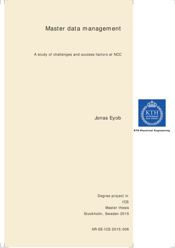
This synchronization can be done in two ways and that is in either passive or active ways. The active way involves sending probing packets through the networks whichcan measure the desired parameters. So, for clock synchronization, this involves measuring the clock time for the transmitting unit and the receiving unit with the purposeof synchronizing them against a common clock like the Coordinated Universal Time(UTC) clock. For the passive approach one does not transmit additional probing packetsacross the network but instead relies upon the regular traffic that is sent to performthe clock synchronization. The passive approach is beneficial since it does not requirethe transmission of additional packets through the network, however, this might alsobe a drawback since the accuracy might be reduced with the reliance on the regularlytransmitted packets [11].2.6Packet delay variation or JitterThe packet delay variation, often referred to as the jitter, is defined as the differencebetween the one-way delay of two consecutive packets. The simple expression for this isas follows,Jitter Delay P acket B Delay P acket A,(3)where packet B arrives directly after packet A. Worth noting is that the jitter disregardsany potential loss that might have occurred in the data transmission since it takesthe one-way delay difference of two consecutive received packets. So if packets aretransmitted in the order of packets A, B, and C, the loss of packet B makes the equationin 3 become, Jitter Delay P acket C Delay P acket A. This kind of behavior meansthat the jitter can almost be seen as a form of a derivative of the delay with it indicatinghow much the delay is changing. The calculation of the jitter can help determine manyproperties of a networks behavior. One of the most important of these properties iswhen the jitter increases in a network this typically indicates that the queues in thenodes, i.e. routers or switches, are increasing.To properly visualize the jitter one must plot it against the received indexes andnot care about the packet number as seen in figure 4, this is in contrast to how the delayis displayed as seen in section 2.4. What this means is that the jitter must be plottedagainst the receiver’s internal counter that counts the order that the packet has arrivedin; so for instance, if packet 1 arrives followed by packet 10 then the received indexesshould be 0 and 1. The reason for plotting the jitter in this way is due to the fact statedpreviously where the delay difference between two consecutive packets is what definesthe jitter. So, one can say that the jitter does not care about which order that thepackets should be received in but rather the order that they actually are received in.11

Figure 4: A plot over the jitter against received index for a stream set measurementthat is of a single user 2.4 GHz WLAN with high quality transmission character. Moreinformation about this can be seen in sections 3.1 and 3.2.As for the delay in section 2.4 a histogram over the jitter in figure 4 can be plottedas seen in figure 5. However, in the case of the jitter this does not prove to give thatmuch information since the jitter by its nature will probably be pending around 0 forthe whole transmission, if this would not be the case then the delay would always beincreasing or decreasing in an uncontrolled manner. This behavior makes it so that thejitter histogram for the entire transmission will almost always also be around 0 as seenin figure 5.12

Figure 5: A Histogram over the jitter for a stream set measurement that is of a singleuser 2.4 GHz WLAN with high quality transmission character. More information aboutthis can be seen in sections 3.1 and 3.2.To be able to properly utilize jitter histograms it proves to be much better to use slidingwindows, as talked about in the bandwidth section 2.3, where the histograms are doneon parts of the jitter in figure 4. The result of doing this can be seen in figure 6. Inthis kind of a plot, the sliding window captures all the jitter values for a certain timeframe, creates a histogram, and then moves forward with a specific time frame where itrepeats the process. By doing this it becomes easier to see eventual changes in how thedistribution of the jitter and thus how the delay changes over time. However, to be ableto effectively see these changes it is critical that the right window size is chosen; if it istoo large then the histograms becomes less sensitive to rapid changes whereas if it is tosmall it might become too sensitive. In a similar manner, the sliding window step sizehas to be selected with care. Too large of a step size and critical information might bemissed and too small of a step size might lead to a large number of histograms, makingthe plot difficult to interpret and demanding for most computers to process. All of the13

histograms that are created are normalized with regard to how many jitter elementsthere are in a specific histogram, thus making the maximum possible value for a jitterbin equal to one.Figure 6: Multiple histograms created over the jitter seen in figure 4. Here the slidingwindow has a size of 1 second and is moved forward in increments of 1/5 of a second.Each histogram covers the range of [-100000 100000] microseconds and is segmented into5000 bins.2.7Packet lossThe packet loss can be defined as the packets which are lost when traveling from thetransmitter to the receiver in a packet switched network. As said in section 2.4 the losscan be seen as a packet with infinite delay, thus the packet will never arrive at its desireddestination. The amount of packet loss can be calculated by taking the number of sentpackets divided by the number of received packets, with a value of 1 indicating thatall packets were successfully received and a value

D armed s a g ar denna rapport ut p a att unders oka hur olika tr adl osa n atverk beter sig n ar n atverksf orh allandena varierar och n ar data skickas p a olika s att via UDP. De tr adl osa n atverk som unders oks ar: 2.4 GHz WLAN (Wireless Local Area Net-work), 5.0 GHz WLAN och 4G. F or att unders oka hur dessa n atverk beter sig s a m aste