WIXLIB

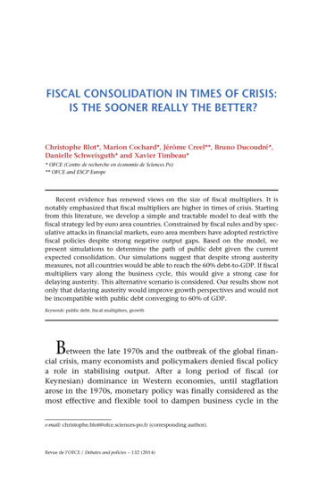
Economics: The Open-Access, Open-Assessment E-Journal 13 (2019–42)Table 1: Regional non-compliance with fiscal targets (2009 2016)Non-compliance withthe spending ruleNon-compliance with deficit riasCantabriaCastilla-LaManchaCastilla yLeonCataluñaComunidad2009201020112012 2013 20142015 20162014 20152016 Non-compliance with thedebt target20132014 20152016 ValencianaExtremadura GaliciaMadridMurciaNavarraPaís VascoLa Rioja Source: AIReF (2018)3Empirical analysis I: A standard econometric approachThe departure point of the first econometric analysis is the following AR (2) model:GALt β0 β1 SPAINt β2 GALt 1 β3 GALt 2 εt(1)In Equation (1), the variables GAL and SPAIN are inter-annual real GDP growth rates ofGalicia and Spain, respectively. 5 The data for the former are from the Galician Institute ofStatistics (www.ige.eu), and the data for Spain are from the National Institute of Statistics(www.ine.es). In both cases, we rely on the quarterly seasonally adjusted data provided on thewebsites. We use Eviews 10.5 for the econometric estimates.The estimation period is 1996:Q1 to 2008:Q4. The selection of the starting point is based onthe evidence provided by Lago-Peñas (2001), who shows that the synchrony of the Spanish and5 Defined as the variation of GDP in each quarter in relation to the same quarter of the previous year.www.economics-ejournal.org6

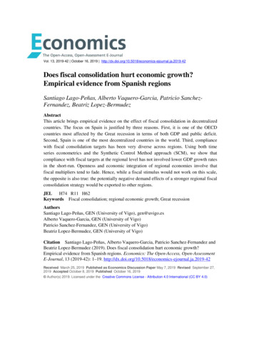
Economics: The Open-Access, Open-Assessment E-Journal 13 (2019–42)Galician business cycles has substantially converged since the early 1990s. Therefore, thegoodness of fit will tend to be significantly higher, while the sample size is large enough toperform estimates. Two lags for the variable GAL are enough to capture the dynamics. 6 To ruleout specification problems, we perform two complementary tests on the specification. First, aHausman test on the endogeneity of the variable SPAIN’s p-value of the corresponding Waldtest is high (p-value 0.25) and thus the null hypothesis of exogeneity is not rejected. 7 Second, aGranger causality test is performed to verify the causation order. The results in Table 2 clearlyshow that we can reject the null hypothesis of no causation from SPAIN to GAL (pvalue 0.001) but not the opposite causation (p-value 0.88).Table 3 reports the ordinary least squares (OLS) estimate of Equation (1). The fit is good(R2 0.853). The null hypothesis of no autocorrelation cannot be discarded according to theBreusch–Godfrey serial test (p-value 0.12). The corresponding correlogram yields the sameconclusion. Both SPAIN and the first lag of GAL, but not the second one, are highly significantvariables, with coefficients around 0.6.Our econometric results allow us to forecast the Galician GDP growth rate from 2009 to2017. In particular, using observed data for the variable SPAIN, we perform a dynamic forecastassuming that the relationship estimated in Table 2 will hold. Figure 4 shows both series. Theobserved GDP growth is clearly above the forecasted growth throughout the period 2009–2014.The sign of the differential changes at the end of 2014, when the forecasted growth exceeds theobserved growth. Hence, in 2015 and 2016, the Galician GDP growth rate was slower that itshould be, taking into account the recovery of the Spanish economy. The situation changesagain at the end of 2016 when the two series overlap. Moreover, in 2017, the observed GDPgrowth rate is slightly higher than that forecasted.In sum, looking at the whole period, the observed GDP growth rate is significantly abovethe forecasted rate. Hence, the data do not support the existence of a price to pay for fiscalconsolidation in terms of short-run GDP growth. 8Table 2: Granger causality test. Period 1996Q1 2008Q4.Null hypothesisp-valueSPAIN does not Granger cause GAL0.0002***GAL does not Granger cause SPAIN0.89Notes: 2 lags included. *** p-value 0.01. Source: Authors’ elaboration.6 Adding the first lag of SPAIN and the third one of GAL on the right-hand side does not improve the fitness,reducing the adjusted R2. According to a joint Wald test, their coefficients are not significantly different from zero (pvalue 0.17).7 The test is implemented in two steps. First, SPAIN is regressed on its own first two lagged values and the twolagged values of GAL. The residuals obtained are included in the original equation. The null hypothesis is that theyare not statistically significant.8 This conclusion holds if we discount the most relevant positive asymmetric shock affecting the Galician economyduring the period, the Jacobean year 2010. According to BBVA research (2010), the Galician GDP growth rate wouldhave been 0.5–0.6% higher in 2010, 0.2% higher in 2011 and 0.1% higher in 2012 thanks to the impact of theJacobean year on tourism.www.economics-ejournal.org7

Economics: The Open-Access, Open-Assessment E-Journal 13 (2019–42)Table 3: Econometric estimate of equation (1)0.65***SPAIN(6.55)0.60***GAL-1(4.45) 0.11GAL-2( 0.91)R20.853Endogeneity Hausman test (p-value)0.25B-G serial correlation LM test (p-value)0.12Number of observations50Notes: t-statistics in parenthesis. *** p-value 0.01 Source: Authors’ elaboration.Figure 4: Observed and forecasted Galician GDP growth rates using specification 162017FORECASTEDSource: Authors’ own elaboration4Empirical analysis II: The synthetic control method approachThe synthetic control method (SCM) is based on the seminal contribution by Abadie andGardeazabal (2003), who analyse the effects of terrorism in the Basque Country. The SCM isrefined in subsequent works by Abadie et al. (2010) on the effects of the anti-tobacco law inCalifornia and Abadie et al. (2015) on the costs of reunification in Germany.The SCM analyses the consequences of a specific event or intervention in a region bycomparing the observed data with what would have happened in the absence of the intervention.Insofar as it requires the creation of a counterfactual, the first step of the method is to find othersimilar regions that remained unaffected by the event (the comparison units) and merge them towww.economics-ejournal.org8

Economics: The Open-Access, Open-Assessment E-Journal 13 (2019–42)create a synthetic region close to the case of interest. More formally, the SCM supposes thatthere are J 1 regions or “units”, where j 1 is the “treated unit” and units j 2 to j J 1 constitutethe “donor pool” (Abadie et al., 2010: 493–505). Following Abadie et al. (2010) and Abadie etal. (2015), we assume that the sample is a balanced panel and includes a positive number of preintervention periods, T0, as well as a positive number of post-intervention periods, T1, withT T1 T0.The synthetic control is defined as a weighted average of the units in the donor poolrepresented by a (J 1) vector of weights W (w2, .,wJ 1), with 0 wj 1 for j 2, .J andw2 . wJ 1 1. Choosing a particular value for W is equivalent to choosing a synthetic control.Let X1 be a (k 1) vector containing the values of the pre-intervention characteristics of thetreated unit that we aim to match as closely as possible, and let X0 be the k J matrix collectingthe values of the same variables for the units in the donor pool. The pre-interventioncharacteristics in X1 and X0 may include the pre-intervention values of the outcome variable.The difference between the pre-intervention characteristics of the treated unit and asynthetic control is given by the vector X1 X0W. As in the research by Abadie et al. (2010) andAbadie et al. (2015), we select the synthetic control, W*, that minimizes the size of thisdifference. This can be operationalized in the following manner. For m 1, ., k, let X1m be thevalue of the m th variable for the treated unit and let X0m be a 1 J vector containing the valuesof the m-th variable for the units in the donor pool. Abadie et al. (2015) choose W* as the valueof W that minimizes: 𝑘𝑚 1 𝑣𝑚 (𝑋1𝑚 𝑋0𝑚 𝑊)2(2)where vm is a weight that reflects the relative importance assigned to the m-th variables whenwe measure the discrepancy between X1 and X0W. Of course, it is crucial that the syntheticcontrol closely reproduces the values that the variables with large predictive power over theoutcome of interest take for the treated unit. Accordingly, those variables should be assignedlarge vm weights. In the empirical application below, we apply a cross-validation method tochoose vm.Let Yjt be the outcome of unit j at time t. In addition, let Y1 be a (T1 1) vector collecting thepostintervention values of the outcome for the treated unit. That is, Y1 (Y1To 1, , Y1T)’.Similarly, let Y0 be a (T1 J) matrix, where column j contains the post-intervention values of theoutcome for unit j 1. The synthetic control estimator of the effect of the treatment is given bythe comparison of post-intervention outcomes between the treated unit, which is exposed to theintervention, and the synthetic control, which is not exposed to the intervention, Y1-Y0W*. Thatis, for a post-intervention period t (with t T0), the synthetic control estimation of the effect ofthe treatment is given by the comparison between the outcome for the treated unit and theoutcome for the synthetic control in that period:𝐽 1𝑌1𝑡 𝑤𝑗 𝑌𝑗𝑗𝑗 2The matching variables in X0 and X1 are meant to be predictors of post-interventionoutcomes. These predictors are themselves not affected by the intervention. To choose thewww.economics-ejournal.org9

Economics: The Open-Access, Open-Assessment E-Journal 13 (2019–42)weights vm in Equation (2), a cross-validation technique is used, following Abadie et al. (2015);these weights minimize the root mean square prediction error:𝑇0𝐽 1𝑡 1𝑗 221/21𝑅𝑅𝑆𝑃𝑃 𝑌1𝑡 𝑤𝑗 𝑌𝑗𝑗 𝑇0In our case, the variables used for the SCM are reported in Table 4. We include variables ondemography, the labour market, human capital, physical capital (both public infrastructure andprivate), exports and foreign investment inflows, poverty (AROPE), competitiveness (theRegional Competitive Index or RCI computed by the European Commission) and the sectorialstructure. While in most cases we use average values over the pre-treatment period, data for theyear 2008 are used for some variables. 9 The sample covers the period 1995–2016 for the 17Table 4: SCM variablesDefinitionDatabaseVariablePer capita GDPPopulationVariation of populationPopulation over 64Secondary educationSuperior educationEmploymentUnemploymentAROPERegional per capita GDP expressed in % of Spanishper capita GDP in 2008Share of regional population over total SpanishpopulationPrivate capital stockAnnual variation rate of regional populationShare of population over 64 years oldShare of active population with secondary level studiesShare of active population with higher level studiesEmployed over population between 16 and 64Unemployment rateRate of risk of poverty or social exclusion in 2008Stock of private productive capital in 2008. Figures inthousands of constant euro base 2010 per employee.Public capital stockStock of public productive capital in 2008. Figures inthousands of constant 2005 base euro per employee.Primary sectorIndustryConstructionServicesExportsForeign InvestmentRCIShare of primary sector over total GDPShare of industry over total GDPShare of construction over total GDPShare of services over total GDPExports over GDPForeign investment received over GDPRegional competitiveness index in 2008 computed bythe European CommissionFEDEA (2018)INE (2018)INE (2018)INE (2018)IVIE (2018a)IVIE (2018a)FEDEA (2018)FEDEA (2018)INE (2018)IVIE (2018b)IVIE (2018b)INE (2018)INE (2018)INE (2018)INE (2018)DataComEx (2018)DataInvEx (2018)EC (2018)Source: Average values over the period 1995 2008, unless expressly indicated. Authors’ elaboration.9 In the case of variable AROPE and the RCI due to availability of data. In the case of both private and public capitalbecause of the stock nature of variables.www.economics-ejournal.org10

Economics: The Open-Access, Open-Assessment E-Journal 13 (2019–42)Spanish regions. We choose the weights vm to minimize the root mean square prediction errorover the validation period. Table 5 shows the computed weights, which are those used to createthe “synthetic Galicia”, for which the values are collected together with the correspondingactual values in Table 6.Table 5: SCM regional iasCantabriaCastilla y LeonCastilla-La ManchaCataluñaComunidad ValencianaExtremaduraMadridMurciaNavarraPaís VascoLa urce: Authors’ elaboration.Table 6: SCM estimation resultsPer capita GDPPopulationVariation of populationPopulation over 64Secondary educationSuperior educationEmploymentUnemploymentAROPEPrivate capital stockPublic capital stockPrimary sectorIndustryConstructionServicesExportsForeign 045.20Synthetic 4,9853,3960.0630.190.100.640.110.006743.65Source: Authors’ elaboration.www.economics-ejournal.org11

Economics: The Open-Access, Open-Assessment E-Journal 13 (2019–42)Figure 5: Observed and SCM forecasted Galician GDP growth 20152016FORECASTEDSource: Authors’ own elaborationFigure 5 shows both the observed and the synthetic growth rates of Galicia for the period2009 to 2016. Except for the years 2009 and 2011, the negative observed values are lower andpositive growth rates are higher than in the counterfactual.Figure 6 presents the previous annual growth rates. In both cases, the value is negative, butthe actual rate ( 2.30%) is clearly lower in absolute terms than that corresponding to thesynthetic unit ( 3.91%).Figure 7 shows both the actual and the synthetic values of the variation rates of the GDP forGalicia from 1995 to 2016. While most of the actual values are lower before 2008, since thenthey have been higher than the synthetic estimate of the region’s growth. This again supports theidea that fiscal austerity implemented to meet the deficit targets has not involved an evidentprice in terms of regional economic growth.To check the robustness of the results, we replicate the analysis, constraining the donorregions to those in which the deviation from the fiscal consolidation targets has been wider(Castilla-La Mancha, Cataluña, Comunidad Valenciana and Murcia). The regional weights thatminimize the root mean square prediction error (RMSPE 0.0071) over the validation period are0.791 for Cataluña and 0.219 for Castilla-La Mancha. Figure 8 shows the new results. Over theperiod 2004–2012, the growth of the counterfactual of Galicia is below the actual growth. After2013, the values are slightly higher, but the positive gap in the counterfactual in recent yearsdoes not compensate for the negative gap in 2012.www.economics-ejournal.org12

Economics: The Open-Access, Open-Assessment E-Journal 13 (2019–42)Figure 6: Cumulative observed and forecasted GDP growth RECASTEDSource: Authors’ own elaborationFigure 7: Observed and SCM GDP growth rates over the period 1995 2016Source: Authors’ own elaborationwww.economics-ejournal.org13

Economics: The Open-Access, Open-Assessment E-Journal 13 (2019–42)Figure 8: Observed and constrained SCM GDP growth rates over the period 1995 2016Source: Authors’ own elaboration5ConclusionsRegional governments provide a convenient field to test whether fiscal consolidation involves aprice to pay in terms of the short-run GDP growth rate. Given the high fiscal decentralization inSpain, the depth of the effects of the Great Depression on the public accounts at the regionallevel in Spain and the diversity of commitments to fiscal targets, this country is the best casestudy among the OECD members.To perform the test, we focused our attention on the region showing a better performance interms of compliance of the fiscal targets agreed with the European Commission. In particular,we compare the observed short-run GDP growth rates with two simulations. The first one isbased on the estimate of a time-series model relating the GDP dynamics of Galicia and Spainover the period 1995–2008. The second one relies on the more sophisticated synthetic controlmethod (SCM) approach. In both cases, we show that stricter fiscal consolidation has notproduced a significant reduction in economic growth. Indeed, the economic performance ofGalicia would have been slightly better than expected using both methodologies.Our interpretation of the results is closely related to the traditional theory of fiscalfederalism (Musgrave, 1959). According to it, openness and economic integration of regionaleconomies involve fiscal multipliers that tend to fade. A fiscal stimulus would not work on thisscale. Our results show that the opposite is also true: the potentially negative demand effects ofa stronger regional fiscal consolidation strategy would be exported to other regions.www.economics-ejournal.org14

Economics: The Open-Access, Open-Assessment E-Journal 13 (2019–42)The most relevant policy implication of our results is that decentralization could indeedcontribute to the compliance with fiscal consolidation plans on the national scale, reversing theusual arguments on both the common pool’s problem affecting fiscal stability in decentralizedcountries and the challenge involved by “soft budget constraints” and bailout expectations(Goodspeed, 2017). If the negative demand effects of regional fiscal consolidation are mostlyexported to other regions, one of the reasons most often argued to delay deficit cuts andcompliance with fiscal targets is deactivated.The smartest strategy for all regions is to cut deficit, getting the benefits and exporting thecosts in terms of lower GDP growth rates. But if decentralization is

need for fiscal consolidation, Spain is the best candidate among the OECD members. In short, our analysis is based on the short-run GDP dynamics of the regional leader in the compliance with fiscal consolidation targets (Galicia) and compares the observed GDP growth rates with what would have happened with softer regional fiscal consolidation.