WIXLIB

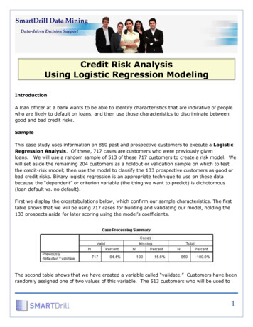
Credit Risk AnalysisUsing Logistic Regression ModelingIntroductionA loan officer at a bank wants to be able to identify characteristics that are indicative of peoplewho are likely to default on loans, and then use those characteristics to discriminate betweengood and bad credit risks.SampleThis case study uses information on 850 past and prospective customers to execute a LogisticRegression Analysis. Of these, 717 cases are customers who were previously givenloans. We will use a random sample of 513 of these 717 customers to create a risk model. Wewill set aside the remaining 204 customers as a holdout or validation sample on which to testthe credit-risk model; then use the model to classify the 133 prospective customers as good orbad credit risks. Binary logistic regression is an appropriate technique to use on these databecause the “dependent” or criterion variable (the thing we want to predict) is dichotomous(loan default vs. no default).First we display the crosstabulations below, which confirm our sample characteristics. The firsttable shows that we will be using 717 cases for building and validating our model, holding the133 prospects aside for later scoring using the model’s coefficients.The second table shows that we have created a variable called “validate.” Customers have beenrandomly assigned one of two values of this variable. The 513 customers who will be used to1

build the model are assigned a value of 1. The remaining 204 customers will be assigned avalue of zero, and will constitute the validation sample on which the model will be tested.The crosstabulations also show that the modeling sample contains 410 customers who did notdefault on a previous loan, and 103 who did default. The validation or holdout sample contains163 customers who did not default, and 41 who did.Logistic Regression AnalysisNow we will run a logistic regression modeling analysis and examine the results. Our model willbe testing several candidate predictors, including: AgeLevel of educationNumber of years with current employerNumber of years at current addressHousehold income (in thousands)Debt-to-income ratioAmount of credit card debt (in thousands).Our logistic regression modeling analysis will use an automatic stepwise procedure, which beginsby selecting the strongest candidate predictor, then testing additional candidate predictors, oneat a time, for inclusion in the model. At each step, we check to see whether a new candidatepredictor will improve the model significantly. We also check to see whether, if the newpredictor is included in the model, any other predictors already in the model should stay or beremoved. If a newly entered predictor does a better job of explaining loan default behavior,then it is possible for a predictor already in the model to be removed from the model because itno longer uniquely explains enough. This stepwise procedure continues until all the candidatepredictors have been thoroughly tested for inclusion and removal. When the analysis is finished,2

we have the following table that contains various statistics.For our purposes here, we can focus our attention on the “B” column, the “Sig.” column and the“Exp(B)” column, explained below.The table's leftmost column shows that our stepwise model-building process included foursteps. In the first step, a constant as well as the debt-to-income-ratio predictor variable(“debtinc”) are entered into the model. At the second step the amount of credit card debt(“creddebt”) is added to the model. The third step adds number of years at current employer(“employ”). And the final step adds number of years at current address (“address”).The “B” column shows the coefficients (called Beta Coefficients, abbreviated with a “B”)associated with each predictor. We see that number of years at current employer and numberof years at current address have negative coefficients, indicating that customers who have spentless time at either their current employer or their current address are somewhat more likely todefault on a loan. The predictors measuring the debt-to-income ratio and amount of credit carddebt both have positive coefficients, indicating that higher debt-to-income ratios or higheramounts of credit card debt are associated with a greater likelihood of defaulting on a loan.The “Sig.” column shows the levels of statistical significance associated with the variouspredictors in the model. The numbers essentially show us the likelihood that the predictor’s3

coefficient is spurious. The numbers are probabilities expressed as decimals. We want thesenumbers to be small, and they are, giving us our first indication that we appear to have a goodmodel.For example, the value of 0.018 associated with number of years at current address indicatesthat we would expect our model’s result to deviate significantly from reality only about 18 timesout of a thousand if we repeated our model-building process over and over again on new datasamples. The statistical significance levels associated with the other three predictors are allsmaller than 0.001 (one chance in a thousand of a spurious result), and so they are shownsimply as 0.000.While the “B” column is convenient for testing the usefulness of predictors, the “Exp(B)” columnis easier to interpret. Exp(B) represents the ratio-change in the odds of the event of interest fora one-unit change in the predictor. For example, Exp(B) for number of years with currentemployer is equal to 0.769, which means that the odds of default for a person who has beenemployed at their current job for two years are just 0.769 times the odds of default for a personwho has been employed at their current job for 1 year, all other things being equal.Once a final model is created and validated, the information in the above table can be used toscore the individual cases in a prospect database. This will allow the bank’s marketingdepartment to focus their acquisition efforts on those prospects that have the lowest modelpredicted probability of defaulting on a loan. It is a simple matter to generate computerreadable instructions that can be used to quickly do the file scoring.After building a logistic regression model, we need to determine whether it reasonablyapproximates the behavior of our data. There are usually several alternative models that passthe diagnostic checks, so we need tools to help us choose between them. Here are three typesof tool that help ensure a valid model:Automated Variable Selection. When constructing a model, we generally want to include onlypredictors that contribute significantly to the model. The modeling procedure that we used offersseveral methods for stepwise selection of the "best" predictors to include in the model, and weused one of these stepwise methods (Forward Selection [Likelihood Ratio]) to automaticallyidentify our final set of predictors.However, since we used a stepwise variable-selection procedure, the significance levelsassociated with the model predictors may be somewhat inaccurate because they are assuming asingle-step process rather than a multi-step process. So we also use additional diagnostics togive us more confidence in our model.Pseudo R-Squared Statistics. The well-known r-squared statistic, which measures thevariability in the dependent variable that is explained by a linear regression model, cannot becomputed for logistic regression models because our dependent variable is dichotomous rather4

than continuous. So we instead use what are called pseudo r-squared statistics. The pseudo rsquared statistics are designed to have similar properties to the true r-squared statistic. Thetable below shows that as our stepwise procedure moved forward from step one to step four, thepseudo r-squared statistics became progressively stronger. For those who are familiar with ther-squared statistic from linear regression, the Nagelkerke statistic in the far righthand columnrepresents a good approximation to that statistic, having a maximum possible value of 1.00. Itshows that approximately 72% of the variation in the dependent variable is explained by thefour predictors in our final model.We also test the model’s goodness-of-fit using additional diagnostics (not shown here), andthese additional tests also confirm that we have a good model.Classification and Validation. Crosstabulating observed response categories with predictedcategories helps us to determine how well the model identifies defaulters. Here is aclassification and validation crosstabulation table:5

The table shows that the model correctly classified about 96% of the modeling sample’s nondefaulters and about 76% of the modeling sample’s defaulters, for an overall correctclassification percentage of about 92%. Similarly, when applied to the holdout or validationsample, the model correctly identified about 95% of the non-defaulters and about 81% of thedefaulters, for an overall correct classification percentage of about 92%.The double-panel graph below provides additional information about the model’s strength. Itshows probability distributions for the probability of defaulting, separately for actual nondefaulters and actual defaulters. The binary logistic regression model assigns probabilities ofdefaulting to each customer, ranging from zero to 1.00 (zero to 100%). In this case, it uses acut point of exactly 0.50 (50% probability) as the dividing line between predicted non-defaultersand predicted defaulters.6

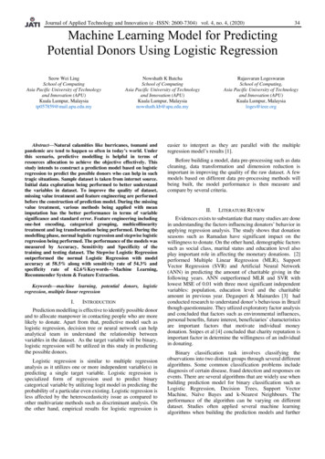
The leftmost graph shows that the modeling process assigned the bulk of the actual nondefaulters very low probabilities of defaulting, far below the 50% probability cut point. And therighthand graph shows that the model assigned the bulk of the defaulters very high probabilitiesof defaulting, far above the 50% cut point. So this adds more confirmation that we have a goodmodel.Now that we have a valid predictive model, we can use it to score a prospect file. The graphbelow shows the result after we have scored our 133 prospects.7

It shows that approximately 67% of the prospects would not be expected to default on aloan. (If we had used much larger customer and prospect samples, as would typically be thecase, then the prospect sample’s results would more closely resemble the modeling sample’sresults.) Note that the separation of prospects into predicted defaulter and non-defaultersubgroups is not quite as clean as for the modeling sample. Although larger samples wouldmitigate this difference, it is typical for a model to deteriorate slightly when applied to a samplethat is different from the one on which the model was built, due to natural sampling error.A critical issue for loan officers is the cost of what statisticians refer to as Type I and Type IIerrors. That is, what is the cost of classifying a defaulter as a non-defaulter (Type I error)? Andwhat is the cost of classifying a non-defaulter as a defaulter (Type II error)?If bad debt is the primary concern, then we want to lower our Type I error and maximize our“sensitivity”. (Sensitivity is the probability that a "positive" case [a defaulter] is correctly8