Transcription
Multilevel Logistic RegressionEdps/Psych/Soc 587Carolyn J. AndersonDepartment of Educational Psychologyc Board of Trustees, University of IllinoisSpring 2020
Overview Logistic Reg Binomial Dist Systematic Link 2 Approaches Pop Mod Random Effects Cool 3 Levels IRT Wrap-upOutlineIn this set of notes:Example Data SetsQuick Introduction to logistic regression.Marginal Model: Population-Average ModelRandom Effects Model: Subject-specific Model3-level multilevel logistic regressionReading/References:Snijders & Bosker, Chapter 14Molenberghs, G. & Verbeke, G. (2005). Models for DiscreteLongitudinal Data. Springer.Agresti, A. (2013). Categorical Data Analsysi, 3rd Edition. Wiley.Agresti, A. (2019). Introduction to Categorical Data Analysis, 3rdedition. Wiley. (included R and SAS code).C.J. Anderson (Illinois)Multilevel Logistic RegressionSpring 20202.2/ 130
Overview Logistic Reg Binomial Dist Systematic Link 2 Approaches Pop Mod Random Effects Cool 3 Levels IRT Wrap-upMore ReferencesSkrondal, A. & Rabe-Hesketh, S. (2004). Generalized Latent VariableModeling. NY: Chapman & Hall/CRC.de Boeck, P. & Wilson, M. (editors) (2004). Explanatory ItemResponse Models. Springer.Molenbergahs, G. & Verbeke, G. (2004). An introduction to(Generalized Non) Linear Mixed Models, Chapter 3, pp 11-148. In deBoeck, P. & Wilson, M. (Eds.) Explanatory Item Response Models.Springer.C.J. Anderson (Illinois)Multilevel Logistic RegressionSpring 20203.3/ 130
Overview Logistic Reg Binomial Dist Systematic Link 2 Approaches Pop Mod Random Effects Cool 3 Levels IRT Wrap-upDataClustered, nested, hierarchial, longitudinal.The response/outcome variable is dichotomous.Examples:Longitudinal study of patients in treatment for depression: normal orabnormalResponses to items on an exam (correct/incorrect)Admission decisions for graduate programs in different departments.Longitudinal study of respiratory infection in childrenWhether basketball players make free-throw shots.Whether “cool” kids are tough kids.othersC.J. Anderson (Illinois)Multilevel Logistic RegressionSpring 20204.4/ 130
Overview Logistic Reg Binomial Dist Systematic Link 2 Approaches Pop Mod Random Effects Cool 3 Levels IRT Wrap-upRespiratory Infection DataFrom Skrondal & Rabe-Hesketh (2004) also analyzed by Zeger &Karim (1991), Diggle et. al (2002), but originally from Sommer et al(1983)Preschool children from Indonesia who were examined up to 6consecutive quarters for respiratory infection.Predictors/explanatory/covariates:Age in monthsXeropthalmia as indicator of chronic vitamin A deficiency (dummyvariable)— night blindness & dryness of membranes dryness ofcornea softening of corneaCosine of annual cycle (ie., season of year)Sine of annual cycle (ie., season of year).GenderHeight (as a percent)StuntedC.J. Anderson (Illinois)Multilevel Logistic RegressionSpring 20205.5/ 130
Overview Logistic Reg Binomial Dist Systematic Link 2 Approaches Pop Mod Random Effects Cool 3 Levels IRT Wrap-upLongitudinal Depression ExampleFrom Agresti (2002) who got it from Koch et al (1977)Comparison of new drug with a standard drug for treating depression.Classified as N Normal and A Abnormal at 1, 2 and 4 J. Anderson (Illinois)Response at Each of 3 Time PointsNNA NAN NAA ANN ANA AAN13931441506022292899152725231532Multilevel Logistic RegressionAAA60286Spring 20206.6/ 130
Overview Logistic Reg Binomial Dist Systematic Link 2 Approaches Pop Mod Random Effects Cool 3 Levels IRT Wrap-up“Cool” KidsRodkin, P.C., Farmer, T.W, Pearl, R. & Acker, R.V. (2006). They’recool: social status and peer group for aggressive boys and girls.Social Development, 15, 175–204.Clustering: Kids within peer groups within classrooms.Response variable: Whether a kid nominated by peers is classified asa model (ideal) student.Predictors: Nominator’sPopularityGenderRaceClassroom aggression levelC.J. Anderson (Illinois)Multilevel Logistic RegressionSpring 20207.7/ 130
Overview Logistic Reg Binomial Dist Systematic Link 2 Approaches Pop Mod Random Effects Cool 3 Levels IRT Wrap-upLSAT6Law School Admissions data: 5 items, N 121.Freqency362111132222222221222126128298C.J. Anderson (Illinois)Multilevel Logistic RegressionSpring 20208.8/ 130
Overview Logistic Reg Binomial Dist Systematic Link 2 Approaches Pop Mod Random Effects Cool 3 Levels IRT Wrap-upGeneral Social SurveyData are responses to 10 vocabulary items from the 2004 GeneralSocial Survey from n 1155 respondents.data vocab;input age educ degree gender wordA wordB wordC wordDwordE wordF wordG wordH wordI wordJ none elementary 0101000101100Possible predictors of vocabulary knowledge:AgeEducationC.J. Anderson (Illinois)Multilevel Logistic RegressionSpring 20209.9/ 130
Overview Logistic Reg Binomial Dist Systematic Link 2 Approaches Pop Mod Random Effects Cool 3 Levels IRT Wrap-upLogistic RegressionThe logistic regression model is a generalized linear model withRandom component: The response variable is binary. Yi 1 or 0 (anevent occurs or it doesn’t). We are interesting in probability thatYi 1; that is, P (Yi 1 xi ) π(xi ).The distribution of Yi is Binomial.Systematic component: A linear predictor such asα β1 x1i . . . βj xkiThe explanatory or predictor variables may be quantitative(continuous), qualitative (discrete), or both (mixed).Link Function: The log of the odds that an event occurs, otherwiseknown as the logit: πi (xi )logit(πi (xi )) log1 πi (xi )The logistic regression model is π(xi )logit(π(xi )) log α β1 x1i . . . βj xki1 π(xi )C.J. Anderson (Illinois)Multilevel Logistic RegressionSpring 202010.10/ 130
Overview Logistic Reg Binomial Dist Systematic Link 2 Approaches Pop Mod Random Effects Cool 3 Levels IRT Wrap-upThe Binomial DistributionAssume that the number of “trials” is fixed and we count the number of“successes” or events that occur.Preliminaries: Bernoulli random variablesX is a random variable where X 1 or 0The probability that X 1 is πThe probability that X 0 is (1 π)Such variables are called Bernoulli random variables.C.J. Anderson (Illinois)Multilevel Logistic RegressionSpring 202011.11/ 130
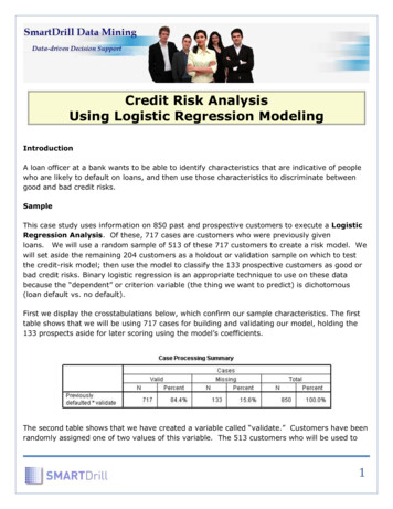
Overview Logistic Reg Binomial Dist Systematic Link 2 Approaches Pop Mod Random Effects Cool 3 Levels IRT Wrap-upBernoulli Random VariableThe mean of a Bernoulli random variable isµx E(X) 1π 0(1 π) πThe variance of X is2var(X) σX E[(X µX )2 ] (1 π)2 π (0 π)2 (1 π) π(1 π)C.J. Anderson (Illinois)Multilevel Logistic RegressionSpring 202012.12/ 130
Overview Logistic Reg Binomial Dist Systematic Link 2 Approaches Pop Mod Random Effects Cool 3 Levels IRT Wrap-upBernoulli Variance vs MeanC.J. Anderson (Illinois)Multilevel Logistic RegressionSpring 202013.13/ 130
Overview Logistic Reg Binomial Dist Systematic Link 2 Approaches Pop Mod Random Effects Cool 3 Levels IRT Wrap-upExample of Bernoulli Random VariableSuppose that a coin is“not fair” or is “loaded”The probability that it lands on heads equals .40 and the probabilitythat it lands on tails equals .60.If this coin is flipped many, many, many times, then we would expectthat it would land on heads 40% of the time and tails 60% of thetime.We define our Bernoulli random variable asX 10if Headsif Tailswhere π P (X 1) .40 and (1 π) P (X 0) .60.Note: Once you know π, you know the mean and variance of thedistribution of X.C.J. Anderson (Illinois)Multilevel Logistic RegressionSpring 202014.14/ 130
Overview Logistic Reg Binomial Dist Systematic Link 2 Approaches Pop Mod Random Effects Cool 3 Levels IRT Wrap-upBinomial DistributionA binomial random variable is the sum of n independent Bernoulli randomvariables. We will let Y represent a binomial random variable and bydefinitionnXY Xii 1The mean of a Binomial random variable isnXXi )µy E(Y ) E(i 1 E(X1 ) E(X2 ) . . . E(Xn )n} {z µx µx . . . µxnz} { π π . π nπC.J. Anderson (Illinois)Multilevel Logistic RegressionSpring 202015.15/ 130
Overview Logistic Reg Binomial Dist Systematic Link 2 Approaches Pop Mod Random Effects Cool 3 Levels IRT Wrap-upVariance of Binomial Random Variable. . . and the variance of a Binomial random variable isvar(Y ) σy2 var(X1 X2 . . . Xn )n} {z var(X) var(X) . . . var(X)nz} { π(1 π) π(1 π) . . . π(1 π) nπ(1 π)Note: Once you know π and n, you know the mean and variance of theBinomial distribution.C.J. Anderson (Illinois)Multilevel Logistic RegressionSpring 202016.16/ 130
Overview Logistic Reg Binomial Dist Systematic Link 2 Approaches Pop Mod Random Effects Cool 3 Levels IRT Wrap-upVariance vs MeanC.J. Anderson (Illinois)Multilevel Logistic RegressionSpring 202017.17/ 130
Overview Logistic Reg Binomial Dist Systematic Link 2 Approaches Pop Mod Random Effects Cool 3 Levels IRT Wrap-upBinomial Distribution Function by ExampleToss the unfair coin with π .40 coin n 3 times.Y number of heads.The tosses are independent of each other.Possible OutcomesX1 X2 X3 Y1 1 1 31 1 0 21 0 1 20 1 1 21 0 0 10 1 0 10 0 1 10 0 0 0C.J. Anderson (Illinois)Probability of a SequenceP (X1 , X2 , X3 )(.4)(.4)(.4) (.4)3 (.6)0 .064(.4)(.4)(.6) (.4)2 (.6)1 .096(.4)(.6)(.4) (.4)2 (.6)1 .096(.6)(.4)(.4) (.4)2 (.6)1 .096(.4)(.6)(.6) (.4)1 (.6)2 .144(.6)(.4)(.6) (.4)1 (.6)2 .144(.6)(.6)(.4) (.4)1 (.6)2 .144(.6)(.6)(.6) (.4)0 (.6)3 .2161.000Multilevel Logistic RegressionProb(Y)P (Y ).0643(.096) .2883(.144) .432.2161.000Spring 202018.18/ 130
Overview Logistic Reg Binomial Dist Systematic Link 2 Approaches Pop Mod Random Effects Cool 3 Levels IRT Wrap-upBinomial Distribution FunctionThe formula for the probability of a Binomial random variable is the number of ways thatP (Y a) P (X 1)a P (X 0)(n a)Y a out of n trials n π a (1 π)n aawhere na n!n(n 1)(n 2) . . . 1 a!(n a)!a(a 1) . . . 1((n a)(n a 1) . . . 1)which is called the “binomial coefficient.”For example, the number of ways that you can get Y 2 out of 3 tosses is 3(2)(1)3 3 22(1)(1)C.J. Anderson (Illinois)Multilevel Logistic RegressionSpring 202019.19/ 130
Overview Logistic Reg Binomial Dist Systematic Link 2 Approaches Pop Mod Random Effects Cool 3 Levels IRT Wrap-upThe Systematic ComponentThe “Linear Predictor”.A linear function of the explanatory variables:ηi β0 β1 x1i β2 x2i . . . βK xKiThe x’s could beMetric (numerical, “continuous”)Discrete (dummy or effect codes)Products (Interactions): e.g., x3i x1i x2iQuadratic, cubic terms, etc: e.g., x3i x22iTransformations: e.g., x3i log(x 3i ), x3i exp(x 3i )Foreshadowing random effects models:ηij β0j β1j x1ij β2j x2ij . . . βKj xKijwhere i is index of level 1 and j is index of level 2.C.J. Anderson (Illinois)Multilevel Logistic RegressionSpring 202020.20/ 130
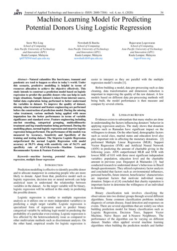
Overview Logistic Reg Binomial Dist Systematic Link 2 Approaches Pop Mod Random Effects Cool 3 Levels IRT Wrap-upThe Link Function:Problem:Probabilities must be between 0 and 1.ηi could be between to .Solution:Use (inverse of) cumulative distribution function (cdf’s) of acontinuous variable to “link” the linear predictor and the mean of theresponse variable.cdf’s are P (random variable specific value), which are between 0and 1Normal “probit” linkLogistic “logit” linkGumbel (extreme value) Complementary log-log linklog[ log(1 π)]C.J. Anderson (Illinois)Multilevel Logistic RegressionSpring 202021.21/ 130
Overview Logistic Reg Binomial Dist Systematic Link 2 Approaches Pop Mod Random Effects Cool 3 Levels IRT Wrap-upSome Example cdf’sC.J. Anderson (Illinois)Multilevel Logistic RegressionSpring 202022.22/ 130
Overview Logistic Reg Binomial Dist Systematic Link 2 Approaches Pop Mod Random Effects Cool 3 Levels IRT Wrap-upPutting All the Components Togetherlog P (Yi 1 xi )P (Yi 0 xi ) logit(P (Yi 1 xi )) β0 β1 x1i β2 x2i . . . βK xKiwhere xi (x0i , x1i , . . . , xKi ).or in-terms of probabilitiesE(Yi xi ) P (Yi 1 xi )exp[β0 β1 x1i β2 x2i . . . βK xKi ] 1 exp[β0 β1 x1i β2 x2i . . . βK xKi ]Implicit assumption (for identification):For P (Yi 0 xi ): β0 β1 . . . βK 0.C.J. Anderson (Illinois)Multilevel Logistic RegressionSpring 202023.23/ 130
Overview Logistic Reg Binomial Dist Systematic Link 2 Approaches Pop Mod Random Effects Cool 3 Levels IRT Wrap-upInterpretation of the ParametersSimple example:P (Yi 1 xi ) exp[β0 β1 xi ]1 exp[β0 β1 xi ]The ratio of the probabilities is the odds(odds of Yi 1 vs Y 0) P (Yi 1 xi ) exp[β0 β1 xi ]P (Yi 0 xi )For a 1 unit increase in xi the odds equalP (Yi 1 (xi 1)) exp[β0 β1 (xi 1)]P (Yi 0 (xi 1))The “odds ratio” for a 1 unit increase in xi equalexp[β0 β1 (xi 1)]P (Yi 1 (xi 1))/P (Yi 0 (xi 1)) exp(β1 )P (Yi 1 xi )/P (Yi 0 xi )exp[β0 β1 xi ]C.J. Anderson (Illinois)Multilevel Logistic RegressionSpring 202024.24/ 130
Overview Logistic Reg Binomial Dist Systematic Link 2 Approaches Pop Mod Random Effects Cool 3 Levels IRT Wrap-upExample 1: Respiratory DataOne with a continuous explanatory variable (for now)Response variableY whether person has had a respiratory infection P (Y 1)Binomial with n 1Note: models can be fit to data at the level of the individual (i.e.,Yi 1 where n 1) or to collapsed data (i.e., i index for everyonewith same value on explanatory variable, and Yi y where n ni ).Systematic componentβ0 β1 (age)iwhere age was been centered around 36 (I don’t know why).Link logitC.J. Anderson (Illinois)Multilevel Logistic RegressionSpring 202025.25/ 130
Overview Logistic Reg Binomial Dist Systematic Link 2 Approaches Pop Mod Random Effects Cool 3 Levels IRT Wrap-upExample 1: The model for respiratory dataOur logit modelexp(β0 β1 (age)i )1 exp(β0 β1 (age)i )We’ll ignore the clustering and use MLE to estimate this model, whichyieldsAnalysis Of Parameter EstimatesStandard95% Conf.ChiPr Parameter EstimateErrorLimitsSquareChiSqIntercept 2.34360.1053 2.55 2.14 495.34 .0001age 0.02480.0056 0.04 0.0119.90 .0001Interpretation: The odds of an infection equals exp( .0248) 0.98 timesthat for a person one year younger.OR The odds of no infection equals exp(0.0248) 1/.98 1.03 times theodds for a person one year older.P (Yi 1 agei ) C.J. Anderson (Illinois)Multilevel Logistic RegressionSpring 202026.26/ 130
Overview Logistic Reg Binomial Dist Systematic Link 2 Approaches Pop Mod Random Effects Cool 3 Levels IRT Wrap-upProbability of InfectionC.J. Anderson (Illinois)Multilevel Logistic RegressionSpring 202027.27/ 130
Overview Logistic Reg Binomial Dist Systematic Link 2 Approaches Pop Mod Random Effects Cool 3 Levels IRT Wrap-upProbability of NO infectionC.J. Anderson (Illinois)Multilevel Logistic RegressionSpring 202028.28/ 130
Overview Logistic Reg Binomial Dist Systematic Link 2 Approaches Pop Mod Random Effects Cool 3 Levels IRT Wrap-upExample 2: Longitudinal Depression DataFrom Agresti (2002) who got it from Koch et al (1977)Model Normal versus Abnormal at 1, 2 and 4 weeks.Also, whether mild/servere (s 1 for severe) and standard/new drug(d 1 for ate-1.3139-0.05960.48241.0174exp β̂0.270.941.622.77Std. Pr χ21 .00010.7885 .0001 .0001The odds of normal when diagnosis is severe is 0.27 times the oddswhen diagnosis is mild (or 1/.27 3.72).For new drug, the odds ratio of normal for 1 week later:exp[ 0.0596 0.4824 1.0174] exp[1.4002] 4.22For the standard drug, the odds ratio of normal for 1 week later:exp[0.4824] 1.62What does exp( 0.0596) exp(0.4824) exp(1.0174) equal?C.J. Anderson (Illinois)Multilevel Logistic RegressionSpring 202029.29/ 130
Overview Logistic Reg Binomial Dist Systematic Link 2 Approaches Pop Mod Random Effects Cool 3 Levels IRT Wrap-upSAS and fitting Logit modelstitle ’MLE ignoring repeated aspect of the data’;proc genmod descending;model outcome diagnose treat time treat*time/ dist bin link logit type3 obstats;output out fitted pred fitvalues StdResChi haberman;Orproc genmod descending;class diagnose(ref First) treat(ref First);* ;model outcome diagnose treat time treat*time/ dist bin link logit type3 obstats;output out fitted pred fitvalues StdResChi haberman;Orproc logistic descending;model outcome diagnose treat time treat*time/ lackfit influence;Can also use the class statement in proc logisticC.J. Anderson (Illinois)Multilevel Logistic RegressionSpring 202030.30/ 130
Overview Logistic Reg Binomial Dist Systematic Link 2 Approaches Pop Mod Random Effects Cool 3 Levels IRT Wrap-upR and fitting Logit modelsSimplest method is to use glm .Suppose the data looks like:id time severe Rx y1000 11100 11200 1.272727.012000000110220220220.012111000001simple glm(y severe Rx time Rx*time,data depress, family binomial)C.J. Anderson (Illinois)Multilevel Logistic RegressionSpring 202031.31/ 130
Overview Logistic Reg Binomial Dist Systematic Link 2 Approaches Pop Mod Random Effects Cool 3 Levels IRT Wrap-upTwo Major Approaches to deal with Clustering“Population-averaged”P (Yij 1 xij ) exp(β0 β1 x1ij . . . βK xKij )1 exp(β0 β1 x1ij . . . βK xKij )Clustering a nuisance.Use generalized estimating equations (GEEs). Only estimate the first 2moments.Random Effects: “subject-specific”P (Yij 1 xij , Uj ) exp(β0j β1j x1ij . . . βKj xKij )1 exp(β0j β1j x1ij . . . βKj xKij )The level 2 model, we specify models for the βkj ’s.The implied marginal of this random effects model when there is only arandom intercept yieldsP (Yij 1 xij ) ZU0C.J. Anderson (Illinois)exp(γ00 γ10 x1ij . . . γK0 xKij U0 )f (U0 )dU01 exp(γ00 γ10 x1ij . . . γK0 xKij U0 )Multilevel Logistic RegressionSpring 202032.32/ 130
Overview Logistic Reg Binomial Dist Systematic Link 2 Approaches Pop Mod Random Effects Cool 3 Levels IRT Wrap-upDemonstration via SimulationThe following random model was simulated:P (Yij 1 xij ) exp(1.0 2.0xij U0j )1 exp(1.0 2.0xij U0j )xij x i ǫij where x i N (0, 4) and ǫij N (0, .01).UO N (0, 4)i.i.d.x i , ǫij and U0j all independent.Number of macro units j 1, . . . , 50.Number of replications (micro units) i 1, . . . , 4.The logit models were fit byMLE ignoring clustering (PROC GENMOD).GEE using “exchangable” correlation matrix (PROC GENMOD)MLE of random effects model (PROC NLMIXED)C.J. Anderson (Illinois)Multilevel Logistic RegressionSpring 202033.33/ 130
Overview Logistic Reg Binomial Dist Systematic Link 2 Approaches Pop Mod Random Effects Cool 3 Levels IRT Wrap-upSimulation: Parameter EstimatesParameterInterceptxMLE IgnoringclusteringStdEstimate ate Error0.5350.3141.3700.293MLE RandomEffectsStdEstimate Error0.8010.4832.2780.543From GEE: correlation .42pFrom Random effects : τ̂o2 2.1636 (s.e. .6018) and τ̂o2 4.6811What do you notice?C.J. Anderson (Illinois)Multilevel Logistic RegressionSpring 202034.34/ 130
Overview Logistic Reg Binomial Dist Systematic Link 2 Approaches Pop Mod Random Effects Cool 3 Levels IRT Wrap-upSimulation: Fitted ValuesC.J. Anderson (Illinois)Multilevel Logistic RegressionSpring 202035.35/ 130
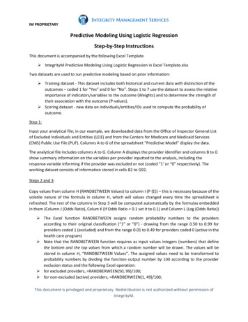
Overview Logistic Reg Binomial Dist Systematic Link 2 Approaches Pop Mod Random Effects Cool 3 Levels IRT Wrap-upConditional vs Marginal ModelsC.J. Anderson (Illinois)Multilevel Logistic RegressionSpring 202036.36/ 130
Overview Logistic Reg Binomial Dist Systematic Link 2 Approaches Pop Mod Random Effects Cool 3 Levels IRT Wrap-upExplanation of Differenceor Why the “population averaged” model (GEE) has weaker effects thanthe random effects model:The subject- (or cluster-) specific or conditional curvesP (Yij 1 xij , U0j ) exhibit quite a bit of variability (& dependencywithin cluster).For a fixed x, there is considerable variability in the probability,P (Yij 1 U0j ).For example, consider x 0, the fitted probabilities range from about.3 to almost 1.0.The average of the P (Yij 1) averaged over j has a less steep“slope”, weaker effect.The greater the variability between the cluster specific curves (i.e. thelarger τ02 and larger correlation within cluster), the greater thedifference.C.J. Anderson (Illinois)Multilevel Logistic RegressionSpring 202037.37/ 130
Overview Logistic Reg Binomial Dist Systematic Link 2 Approaches Pop Mod Random Effects Cool 3 Levels IRT Wrap-upPopulation Averaged ModelHave repeated measures data or nested data correlatedobservations.Use Generalized Estimating Equations (GEE) method (some casesMLE possible)In GLM, we assumed binomial distribution for binary data, whichdetermines the relationship between the mean E(Y ) and the variancevar(Y ) of the response variable.For the GEE part, we need to specify (guess) what the correlationalstructure is for the observations. “working correlation” matrix.Independent: no correlation between observations.Exchangeable: correlation between pairs of observations are same withinclusters (and is the same within all clusters)Autoregressive: for time t and t′ , correlation between Yt and Yt′ equals′ρt tUnstructured: correlations between all pairs within clusters can differC.J. Anderson (Illinois)Multilevel Logistic RegressionSpring 202038.38/ 130
Overview Logistic Reg Binomial Dist Systematic Link 2 Approaches Pop Mod Random Effects Cool 3 Levels IRT Wrap-upThe Working Correlation MatrixGEE assumes a distribution for each marginal (e.g., P (Yij 1) for allj) but does not assume distribution for joint (i.e.,P (Yi1 , Yi2 , . . . , YiN )). . . there’s no multivariate generalizations ofdiscrete data distributions like there is for the normal distribution.Data is used to estimate the dependency between observations withina cluster. (the dependency assumed to be the same within all clusters)Choosing a Working Correlation MatrixIf available, use information you know.If lack information and n is small, then try unstructured to give you anidea of what might be appropriate.If lack information and n is large, then unstructured might requires (too)many parameters.If you choose wrong, thenstill get valid standard errors because these are based on data(empirical).If the correlation/dependency is small, all choices will yield very similarresults.C.J. Anderson (Illinois)Multilevel Logistic RegressionSpring 202039.39/ 130
Overview Logistic Reg Binomial Dist Systematic Link 2 Approaches Pop Mod Random Effects Cool 3 Levels IRT Wrap-upGEE Example: Longitudinal DepressionInterceptdiagnosetreattimetreat*time 0.0280 1.3139 0.1148)(0.1888)Exchangeable 0.0281 (0.1742) 1.3139 (0.1460) 0.0593 (0.2286)0.4825 (0.1199)1.0172 (0.1877)Unstructured 0.0255 (0.1726) 1.3048 (0.1450) 0.0543 (0.2271)0.4758 (0.1190)1.0129 (0.1865)Working correlation for exchangeable .0034Correlation Matrix for Unstructured:Working Correlation MatrixCol1Col2Col3Row11.00000.0747 0.0277Row20.07471.0000 0.0573Row3 0.0277 0.05731.0000(Interpretation the same as when we ignored clustering.)C.J. Anderson (Illinois)Multilevel Logistic RegressionSpring 202040.40/ 130
Overview Logistic Reg Binomial Dist Systematic Link 2 Approaches Pop Mod Random Effects Cool 3 Levels IRT Wrap-upSAS and GEEtitle ’GEE with Exchangeable’;proc genmod descending data depress;class case;model outcome diagnose treat time treat*time/ dist bin link logit type3;repeated subject case / type exch corrw;run;Other correlational structurestitle ’GEE with AR(1)’;repeated subject case / type AR(1) corrw;title ’GEE with Unstructured’;repeated subject case / type unstr corrw;C.J. Anderson (Illinois)Multilevel Logistic RegressionSpring 202041.41/ 130
Overview Logistic Reg Binomial Dist Systematic Link 2 Approaches Pop Mod Random Effects Cool 3 Levels IRT Wrap-upR and GEEInput:model.gee gee(y severe Rx time Rx*time,id, data depress, family binomial, corstr 5.4191Estimated Scale Parameter: 0.985392C.J. Anderson(Illinois)Multilevel Logistic RegressionNumberof 77Robustz-0.1613-9.0016-0.25934.02265.4192Spring 202042.42/ 130
Overview Logistic Reg Binomial Dist Systematic Link 2 Approaches Pop Mod Random Effects Cool 3 Levels IRT Wrap-upR and GEEWorking Correlation[, 1][, 2][1, ] 1.00000 -0.00343[2, ] -0.00343 1.00000[3, ] -0.00343 -0.00343C.J. Anderson (Illinois)[, 3]-0.0034-0.00341.0000Multilevel Logistic RegressionSpring 202043.43/ 130
Overview Logistic Reg Binomial Dist Systematic Link 2 Approaches Pop Mod Random Effects Cool 3 Levels IRT Wrap-upGEE Example 2: Respiratory DataWe’ll do simple (just time) and then complex (lots of predictors):Exchangeable Working CorrelationCorrelation 0.049991012Analysis Of GEE Parameter EstimatesEmpirical Standard Error EstimatesStandard95% ConfidenceParameter EstimateErrorLimitsZIntercept-2.33550.1134 -2.5577 -2.1133 -20.60age-0.02430.0051 -0.0344 -0.0142-4.72Score Statistics For Type 3 GEE AnalysisChiSource DF SquarePr ChiSqage118.24 .0001Estimated odds ratio exp( .0243) 0.96 (or 1/0.96 1.02)Note ignoring correlation, odds ratio 0.98 or 1/0.98 1.03.C.J. Anderson (Illinois)Multilevel Logistic RegressionSpring 2020Pr Z .0001 .000144.44/ 130
Overview Logistic Reg Binomial Dist Systematic Link 2 Approaches Pop Mod Random Effects Cool 3 Levels IRT Wrap-upMarginal Model: Complex ModelExchangeable Working correlation 0.04. . . some model refinement needed . . .Analysis Of GEE Parameter EstimatesEmpirical Standard Error EstimatesParameterEstimate exp(beta) std. ErrorZ Pr Z Intercept 2.420.890.18 13.61 .01age 0.030.970.01 5.14 e1 0.420.660.24 1.77.08female00.001.000.00.cosine 0.570.570.17 3.36 .01sine 0.160.850.15 1.11.27height 0.050.950.03 0.00.C.J. Anderson (Illinois)Multilevel Logistic RegressionSpring 202045.45/ 130
Overview Logistic Reg Binomial Dist Systematic Link 2 Approaches Pop Mod Random Effects Cool 3 Levels IRT Wrap-upMiscellaneous Comments on Marginal ModelsWith GEEThere is no likelihood being maximized no likelihood based tests.(Information criteria statistics: QIC & UQIC)Can do Wald type tests and confidence intervals for parameters. Scoretests are also available.There are other ways to model the marginal distribution(s) of discretevariables that depend on the number of observations per group(macro unit). e.g.,For matched pairs of binary variables, MacNemars test.Loglinear models of quasi-symmetry and symmetry to test marginalhomogeneity in square tables.Transition models.Others.C.J. Anderson (Illinois)Multilevel Logistic RegressionSpring 202046.46/ 130
Overview Logistic Reg Binomial Dist Systematic Link 2 Approaches Pop Mod Random Effects Cool 3 Levels IRT Wrap-upRandom Effects ModelGLM with allow random parameters in the systematic component:ηij β0j β1j x1ij β2j x2ij . . . βKj xKijwhere i is index of level 1 and j is index of level 2.Level 1: Model conditional on xij and Uj :P (Yij 1 xij , Uj ) exp[β0j β1j x1ij β2j x2ij . . . βKj xKij ]1 exp[β0j β1j x1ij β2j x2ij . . . βKj xKij ]where Y is binomial with n 1 (i.e., Bernoulli).Level 2: Model for intercept and slopes:β0j γ00 U0jβ1j γ10 . . . U1j. . . . .βKjC.J. Anderson (Illinois) γK0 UKjMultilevel Logistic RegressionSpring 202047.47/ 130
Overview Logistic Reg Binomial Dist Systematic Link 2 Approaches Pop Mod Random Effects Cool 3 Levels IRT Wrap-upPutting Levels 1 & 2 TogetherP (Yij 1 xij , Uj ) exp[γ00 γ1 x1ij . . . γK xKij U0j . . . UKJ xKJ ]1 exp[γ0 γ1 x1ij . . . γK xKij U0j . . . UKJ xKJ ]Marginalizing gives us the Marginal Model. . .P (Yij 1 xij ) ZU0C.J. Anderson (Illinois).ZUKexp(γ00 γ10 x1ij . . . U0 . . . UK xJij )f (U )dU1 exp(γ00 γ10 x1ij . . . U0 . . . UK xJij )Multilevel Logistic RegressionSpring 202048.48/ 130
Overview Logistic Reg Binomial Dist Systematic Link 2 Approaches Pop Mod Random Effects Cool 3 Levels IRT Wrap-upA Simple Random Intercept ModelLevel 1:P (Yij 1 xij ) exp[β0j β1j x1ij ]1 exp[β0j x1ij ]where Yij is Binomial (Bernoulli).Level 2:β0j γ00 U0jβ1j γ01where U0j N (0, τ02 ) i.i.d.Random effects model for micro unit i and macro unit j:P (Yij 1 xij , U0j ) C.J. Anderson (Illinois)exp[γ00 γ01 x1ij U0j ]1 exp[γ00 γ01 x1ij U0j ]Multilevel Logistic RegressionSpring 202049.49/ 130
Overview Logistic Reg Binomial Dist Systematic Link 2 Approaches Pop Mod Random Effects Cool 3 Levels IRT Wrap-upExample 1: A Simple Random Intercept ModelThe respiratory data of children.The NLMIXED ProcedureSpecificationsData SetDependent VariableDistribution for Dependent VariableRandom EffectsDistribution for Random EffectsSubject VariableOptimization TechniqueIntegration MethodC.J. Anderson (Illinois)WORK.RESPIRErespBinaryuNormalidDual Quasi-NewtonAdaptive GaussianQuadratureMultilevel Logistic RegressionSpring 202050.50/ 130
Overview Logistic Reg Binomial Dist Systematic Link 2 Approaches Pop Mod Random Effects Cool 3 Levels IRT Wrap-upExample 1: Dimensions TableDimensionsObservations UsedObservations Not UsedTotal ObservationsSubjectsMax Obs Per SubjectParametersQuadrature PointsC.J. Anderson (Illinois)Multilevel Logistic Regression1200012002756310Spring 202051.51/ 130
Overview Logistic Reg Binomial Dist Systematic Link 2 Approaches Pop Mod Random Effects Cool 3 Levels IRT W
edition. Wiley. (included R and SAS code). C.J. Anderson (Illinois) Multilevel Logistic Regression Spring 2020 2.2/ 130. . Whether "cool" kids are tough kids. others C.J. Anderson (Illinois) Multilevel Logistic Regression Spring 2020 4.4/ 130 . The response variable is binary. Y i 1or 0(an event occurs or it doesn't). We are .