Transcription
Lecture 8: Heteroskedasticity CausesConsequencesDetectionFixes
Assumption MLR5:Homoskedasticityvar(u x1 , x2 ,., x j ) 2In the multivariate case, this means that thevariance of the error term does not increase ordecrease with any of the explanatory variablesx1 through xj.If MLR5 is untrue, we have heteroskedasticity.
Causes of Heteroskedasticity Error variance can increase as values of anindependent variable increase. Ex: Regress household security expenditures onhousehold income and other characteristics. Variance inhousehold security expenditures will increase as incomeincreases because you can’t spend a lot on securityunless you have a large income.Error variance can increase with extreme valuesof an independent variable (either positive ornegative)Measurement error. Extreme values may bewrong, leading to greater error at the extremes.
Causes of Heteroskedasticity, cont. Bounded independent variable. If Y cannotbe above or below certain values, extremepredictions have restricted variance. (Seeexample in 5th slide after this one.)Subpopulation differences. If you need torun separate regressions, but run a singleone, this can lead to two error distributionsand heteroskedasticity.Model misspecification: form of included variables (square, log, etc.)exclusion of relevant variables
Not Consequences of Heteroskedasticity: MLR5 is not needed to showunbiasedness or consistency of OLSestimates. So violation of MLR5 does notlead to biased estimates.Since R2 is based on overall sums ofsquares, it is unaffected byheteroskedasticity.Likewise, our estimate of root meansquared error is valid in the presence ofheteroskedasticity.
Consequences of heteroskedasticity OLS model is no longer B.L.U.E. (bestlinear unbiased estimator) Other estimators are preferableWith heteroskedasticity, we no longer havethe “best” estimator, because errorvariance is biased. incorrect standard errorsInvalid t-statistics and F statisticsLM test no longer valid
Detection of heteroskedasticity:graphs Conceptually, we know that heteroskedasticitymeans that our predictions have uneven varianceover some combination of Xs. One way to visually check for heteroskedasticity isto plot predicted values against residuals Simple to check in bivariate case, complicated formultivariate models.This works for either bivariate or multivariate OLS.If heteroskedasticity is suspected to derive from asingle variable, plot it against the residualsThis is an ad hoc method for getting an intuitivefeel for the form of heteroskedasticity in yourmodel
Let’s see if the regression from the2010 midterm has heteroskedasticity(DV is high school g.p.a.). reg hsgpa male hisp black other agedol dfreq1 schattach msgpa r mk income1antipeerSource SSdfMS------------- -----------------------------Model 1564.9829711 142.271179Residual 1529.3681 6562 .233064325------------- -----------------------------Total 3094.35107 6573 .470766936Number of obsF( 11, 6562)Prob FR-squaredAdj R-squaredRoot MSE -----------hsgpa Coef.Std. Err.tP t [95% Conf. Interval]------------- -------------male -.1574331.0122943-12.810.000-.181534-.1333322hisp -.0600072.0174325-3.440.001-.0941806-.0258337black -.1402889.0152967-9.170.000-.1702753-.1103024other -.0282229.0186507-1.510.130-.0647844.0083386agedol -.0105066.0048056-2.190.029-.0199273-.001086dfreq1 ach .0216439.00320036.760.000.0153702.0279176msgpa .4091544.008174750.050.000.3931294.4251795r mk .131964.007727417.080.000.1168156.1471123income1 1.21e-061.60e-077.550.0008.96e-071.52e-06antipeer -.0167256.0041675-4.010.000-.0248953-.0085559cons --------------------
Let’s see if the regression from themidterm has heteroskedasticity . . .0-1-2Residuals12. predict gpahat(option xb assumed; fitted values). predict residual, r. scatter residual gpahat, msize(tiny)or . . . rvfplot, msize(tiny)123Fitted values4
Let’s see if the regression from themidterm has heteroskedasticity . . .2. predict gpahat(option xb assumed; fitted values). predict residual, r. scatter residual gpahat, msize(tiny)or . . . rvfplot, msize(tiny)max(uˆ ) 4 yˆ0-1-2Residuals1 123Fitted values4
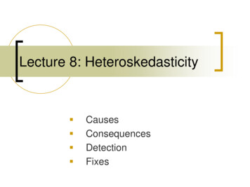
Let’s see if the regression from the2010 midterm has heteroskedasticity This is not a rigorous test forheteroskedasticity, but it has revealed animportant fact: Since the upper limit of high school gpa is 4.0,the maximum residual, and error variance, isartificially limited for good students.With just this ad-hoc method, we stronglysuspect heteroskedasticity in this model.We can also check the residuals againstindividual variables:
2Let’s see if the regression from the2010 midterm has heteroskedasticity. scatter residual msgpa, msize(tiny) jitter(5)or . . . rvpplot msgpa, msize(tiny) jitter(5)same issue0-1-2Residuals1 012msgpa34
Other useful plots for detectingheteroskedasticity twoway (scatter resid fitted) (lowess resid fitted) Same as rvfplot, with an added smoothed line forresiduals – should be around zero.You have to create the “fitted” and “resid” variablestwoway (scatter resid var1) (lowessresid var1) Same as rvpplot var1, with smoothed line added.
Formal tests for heteroskedasticity There are many tests for heteroskedasticity.Deriving them and knowing thestrengths/weaknesses of each is beyond thescope of this course.In each case, the null hypothesis ishomoskedasticity:H 0 : E (u 2 x1 , x2 ,., xk ) E (u 2 ) 2 The alternative is heteroskedasticity.
Formal test for heteroskedasticity:“Breusch-Pagan” test1) Regress Y on Xs and generate squaredresiduals2) Regress squared residuals on Xs (or asubset of Xs)22LM n R3) Calculateû , (N*R ) fromregression in step 2.4) LM is distributed chi-square with k degreesof freedom.5) Reject homoskedasticity assumption if pvalue is below chosen alpha level.2
Formal test for heteroskedasticity:“Breusch-Pagan” test, example After high school gpa regression (not shown):. predict resid, r. gen resid2 resid*resid. reg resid2 male hisp black other agedol dfreq1 schattach msgpa r mk income1 antipeerSource SSdfMSNumber of obs 6574------------- -----------------------------F( 11, 6562) 9.31Model 12.559086211 1.14173511Prob F 0.0000Residual 804.880421 6562.12265779R-squared 0.0154------------- -----------------------------Adj R-squared 0.0137Total 817.439507 6573 .124363229Root MSE ---------------------------------resid2 Coef.Std. Err.tP t [95% Conf. Interval]------------- -------------male -.0017499.008919-0.200.844-.019234.0157342hisp -.0086275.0126465-0.680.495-.0334188.0161637black -.0201997.011097-1.820.069-.0419535.0015541other .0011108.01353020.080.935-.0254129.0276344agedol -.0063838.0034863-1.830.067-.013218.0004504dfreq1 .000406.00034711.170.242-.0002745.0010864schattach -.0018126.0023217-0.780.435-.0063638.0027387msgpa -.0294402.0059304-4.960.000-.0410656-.0178147r mk e1 er .0050848.00302331.680.093-.0008419.0110116cons -------------------
Formal test for heteroskedasticity:Breusch-Pagan test, example. di "LM ",e(N)*e(r2)LM 101.0025. di chi2tail(11,101.0025)1.130e-16 We emphatically reject the null of homoskedasticity.We can also use the global F test reported in theregression output to reject the null (F(11,6562) 9.31,p .00005)In addition, this regression shows that middle school gpaand math scores are the strongest sources ofheteroskedasticity. This is simply because these are thetwo strongest predictors and hsgpa is bounded.
Formal test for heteroskedasticity:Breusch-Pagan test, example We can also just type “ivhettest, nr2” afterthe initial regression to run the LM version of theBreusch-Pagan test identified by Wooldredge. ivhettest, nr2OLS heteroskedasticity test(s) using levels of IVs onlyHo: Disturbance is homoskedasticWhite/Koenker nR2 test statistic: 101.002 Chisq(11) P-value 0.0000 Stata documentation calls this the“White/Koenker” heteroskedasticity test, based onKoenker, 1981.This adaptation of the Breusch-Pagan test is lessvulnerable to violations of the normalityassumption.
Other versions of the Breusch-Pagantest Note, “estat hettest” and “estathettest, rhs” also produce commonlyused Breusch-Pagan tests of the the nullof homoskedasticity, they’re olderversions, and are biased if the residualsare not normally distributed.
Other versions of the Breusch-Pagantest estat hettest, rhs From Breusch & Pagan (1979)Square residuals and divide by mean so that newvariable mean is 1Regress this variable on Xs2 Model sum of squares / 2kestat hettest Square residuals and divide by mean so that newvariable mean is 1Regress this variable on yhat2Model sum of squares / 2 1
Other versions of the Breusch-Pagantest. estat hettest, rhsBreusch-Pagan / Cook-Weisberg test for heteroskedasticityHo: Constant varianceVariables: male hisp black other agedol dfreq1 schattach msgpa r mk income1antipeerchi2(11)Prob chi2 116.030.0000. estat hettestBreusch-Pagan / Cook-Weisberg test for heteroskedasticityHo: Constant varianceVariables: fitted values of hsgpachi2(1)Prob chi2 93.560.0000In this case, because heteroskedasticity is easily detected, ourconclusions from these alternate BP tests are the same, but this is notalways the case.
Other versions of the Breusch-Pagantest We can also use these commands to test whetherhomoskedasticity can be rejected with respect to a subset ofthe predictors:. ivhettest hisp black other, nr2OLS heteroskedasticity test(s) using user-supplied indicator variablesHo: Disturbance is homoskedasticWhite/Koenker nR2 test statistic:2.838 Chi-sq(3) P-value 0.4173. estat hettest hisp black otherBreusch-Pagan / Cook-Weisberg test for heteroskedasticityHo: Constant varianceVariables: hisp black otherchi2(3)Prob chi2 3.260.3532
Tests for heteroskedasticity: White’s test,complicated version1) Regress Y on Xs and generate residuals,square residuals2) Regress squared residuals on Xs, squared Xs,and cross-products of Xs (there will bep k*(k 3)/2 parameters in this auxiliaryregression, e.g. 11 Xs, 77 parameters!)3) Reject homoskedasticity if test statistic (LM orF for all parameters but intercept) isstatistically significant. With small datasets, the number ofparameters required for this test is too many.
Tests for heteroskedasticity: White’s test,simple version1) Regress Y on Xs and generate residuals,square residuals, fitted values, squared fittedvalues2) Regress squared residuals on fitted valuesand squared fitted values:uˆ 0 1 yˆ 2 yˆ v223) Reject homoskedasticity if test statistic (LM orF) is statistically significant.
Tests for heteroskedasticity: White’s test,example. reg r2 gpahat gpahat2Source SSdfMS------------- -----------------------------Model 10.422282825.2111414Residual 807.017224 6571 .122814979------------- -----------------------------Total 817.439507 6573 .124363229Number of obsF( 2, 6571)Prob FR-squaredAdj R-squaredRoot MSE ----------r2 Coef.Std. Err.tP t [95% Conf. Interval]------------- -------------gpahat .0454353.08161190.560.578-.1145505.2054211gpahat2 -.023728.0152931-1.550.121-.0537075.0062515cons ------------------. di "LM ",e(r2)*e(N)LM 83.81793. di chi2tail(2,83.81893)6.294e-19 Again, reject the null hypothesis.
Tests for heteroskedasticity: White’s test This test is not sensitive to normality violationsThe complicated version of the White test can be foundusing the “whitetst” command after running aregression. whitetstWhite's general test statistic : 223.1636Chi-sq(72) P-value 2.3e-17 Note: the degrees of freedom is less than 77 becausesome auxiliary variables are redundant and dropped(e.g. the square of any dummy variable is itself).
In-class exercise Work on questions 1 through 7 on theheteroskedasticity worksheet.
Fixes for heteroskedasticity Heteroskedasticity messes up our variances (and standarderrors) for parameter estimatesSome methods tackle this problem by trying to model theexact form of heteroskedasticity: weighted least squares Requires some model for heteroskedasticity.Re-estimates coefficients and standard errorsOther methods do not deal with the form of theheteroskedasticity, but try to estimate correct variances:robust inference, bootstrapping Useful for heteroskedasticity of unknown formAdjusts standard errors only
Fixes for heteroskedasticity:heteroskedasticity-robust inferencenvar( ˆ ) 2 2(x x) i ii 112xSST 2SSTx, if i2i2 the idealnvar( ˆ1 ) 2 2(x x)uˆi ii 1 robust variance estimatorSSTx2The robust variance estimator is easy to calculatepost-estimation. It reduces to the standard varianceestimate under homoskedasticity.In Stata, obtaining this version of the variance is veryeasy: “reg y x, robust”
Heteroskedasticity-robust inference,example. quietly reg hsgpa male hisp black other agedol dfreq1 schattach msgpa r mk income1antipeer. estimates store ols. quietly reg hsgpa male hisp black other agedol dfreq1 schattach msgpa r mk income1antipeer, robust. estimates store robust. estimates table ols robust, stat(r2 rmse) title("High school GPA models") b(%7.3g)se(%6.3g) t
square residuals, fitted values, squared fitted values 2) Regress squared residuals on fitted values and squared fitted values: 3) Reject homoskedasticity if test statistic (LM