Transcription
VALIDATION OF CFD CODE ANSYS CFX AGAINST EXPERIMENTS WITH SALINE SLUGMIXING PERFORMED AT THE GIDROPRESS 4-LOOP WWER-1000 TEST FACILITYM. Bykov, A. Moskalev, A. Shishov, O. Kudryavtsev, D. PosysaevEDO «GIDROPRESS», Podolsk, RussiaABSTRACTValidation of the CFD code ANSYS CFX was performed in the frame of the experimental and analyticalinvestigations of mixing of coolant flows with different saline concentration fulfilled inEDO “GIDROPRESS” at 4-loop test facility modeling reactor WWER-1000 with the scale 1:5.Calculations were performed with the 3-D code complex ANSYS CFX. The objective of the analyses wasthe code validation with the purpose of further practical implementation.Calculations were performed for the case of experiments with the saline slug in the pump loop seal at theRCP start-up. Unsteady 3-D fields of saline concentration were calculated for the circuit of the facility.Comparison of experimental and predicted data is presented in the paper. Results of CFD analysesdemonstrated very good agreement with the experimental data.1. INTRODUCTIONRIA accidents with the slugs of deborated coolant flow into the core are considered in the safety analysis ofWWER type reactors. These slugs are formed most likely in the RCP loop seals after cessation of naturalcirculation. With the resumption of circulation the slug could be delivered to the core thus causing reactivityinsertion.Mixture of the slug with the rest of the coolant mitigates reactivity effects essentially. A special experimentalprogram was carried out in EDO “GIDROPRESS” to investigate the mixture process of coolant flowscontaining slug with different boron concentration in the flow path upstream the core. A saline (NaCl)solution was used in the reactor model to simulate the slug behavior during the experiments.2. PROBLEM STATEMENTThe objective of this work was validation of the code ANSYS CFX in order to justify its further applicationfor the safety analysis of the WWER type reactors. In the frame of the TACIS project R2.02/02 pre-testcalculations of the velocities, pressure and salt concentration fields in EDO GIDROPRESS’ four-loopexperimental facility scaled 1:5 with regard to WWER-1000 were performed in EDO “GIDROPRESS” usingthe code ANSYS CFX.Calculated results of three following experiments simulating two specific areas of regimes with coolantconvection are presented in this paper:- regimes with leading role of inertia forces characterized by Strouhal criterion; experiment with one RCPactivation- regimes with leading role of gravity force characterized by Froude criterion. Two experiments with theinjection of fluid with different slug densities and coolant flow corresponding to natural circulationconditions. In the first experiment the ratio of the slug density to that of the coolant was equal 1,05, in thesecond experiment – 1,00.3. CALCULATED REGION ELEMENT MESH DEVELOPMENTTo create a solid model Solid Works CAD software was used. The Solid model is required at elaboration ofthe calculated region element mesh that is shown in Figure 1.Because of complex geometry of the flow path, non-structured mesh was used that consists of a fewstructured subregions. Figures 2, 3 and 4 such subregions are shown in different colors. 3-D evaluationmodel of the facility was developed for the CFD simulation of the hydrodynamic processes of boron mixing.Two complexes STAR-CD and ANSYS ICEM CFD were used for mesh development. This mesh consistedof approximately 5 million control cells. In order to check the developed evaluation model test calculationswere performed with the code STAR-CD.
Fig.1: Calculated region element meshFig.2: Inlet nozzle and support tubesFigure 2 shows the mesh in the longitudinal cross-section of the model. The mesh is given here in moredetail in the area of the inlet nozzle and in the area of the lower perforation with support tubes. Figure 3provides the mesh of the lower part of the model in the area of perforation and in the area of measurementsensor location. Figure 4 shows the mesh behind the support tubes in the area of perforated grid and in thearea of coolant evacuation. SST turbulence model was used in all calculations.Fig.3: Part of model in the area of perforation andlocation of transducersFig.4: Perforated grid and outlet nozzle4. EXPERIMENTS DESCRIPTIONThe base of experimental facility is one-to-five scale metal model of WWER-1000 reactor wherein the geometry ofthe flow section of Novovoronezh NPP reactor, Unit No. 5, beginning from inlet nozzles to the core inlet issimulated.The core is simulated partially. Instead of FA simulators and protective tube unit in the reactor model there is an«assembly». The «assembly» is a bundle consisting of 91 tubes with 14х2 mm in diameter that is assembled withthe help of three spacing grids by which the pressure loss of the core and the protective tube unit is simulated. Rodswith conductance measuring sensors are mounted through the model cover into these tubes.The concentrations are measured by electronic conductivity meter "Expert-002" with the limiting admissible basicerror of 2 %, brought to the upper value of the measurement sub-range.
Centrifugal pumps having the following main performances are used as circulating pumps. Each pump has afrequency-controlled drive for the control of volumetric flow. Flow rates in circulation loops are measured with thehelp of electromagnetic flow meters produced by YOKOGAWA Co. with an error of 0,35 % of the current value.In addition, for process purposes, the tapering orifice plates measuring flow rate with an error of 1,5 % are placedin each loop.Initial and boundary conditions are the same for all experiments. The only exceptions are the initial slug volumeand the flowrate in the Loop 4 at steady flow regime. In the initial state the testing bench is filled with water attemperature 20 oC at the atmospheric pressure. The initial concentration of salt in coolant is 0 g/kg. The pumps arenot in operation at Loops 1, 2 and 3. With the help of frequency-controlled pump drive of the Loop 4 the desiredcurve of the flow in the loop Qt is defined (time to reach steady flow is about 15 seconds)(Q t Q o 1 e 0 , 25 t)(1)where:Qо – steady flow rate in the Loop 4;t – time, s.Coolant circulation in the first three loops is realized by reverse flow. The experiment stops on the basis of thesymptom of salt concentration equalization in the reactor model and the circulation loops.The calculation model for ANSYS CFX Code (Figure 5) comprises the model of reactor vessel with eight nozzlesand the model of the pressure part of Loop 4. Additional coordinate system in the Figure 5 is located in thecenter of mass of the saline slug. Figure 6 provides sensor location in the cartogram of the channels (fuelassemblies) in the core model.Fig. 5: Calculation modelFig. 6: Cartogram of sensor locationThe boundary conditions on the flow inlet and outlet were set in accordance with the inlet and outlet nozzles of themodel, respectively. In the first three models the flow inlet and outlet changed their places to model the reverseflow in the loops. The reverse flow rate was assumed to be equal to 10 % of the flow in the loop with the operatingpump. Salt concentration C in the slug in Loop 4 was assumed to be equal to 1 was calculated according to thefollowing formula:C C0(2)C iC1 C 0Where:Ci – current salt concentration at the location of transducer, g/kg;С0 – initial concentration in the loop, g/kg;С1 – concentration of the solution injected into the circuit or initial slug concentration.5. COMPARISON OF CALCULATED RESULTS WITH THE EXPERIMENTAL DATAEvaluation model was imported into the CFD code ANSYS CFX with the help of complex ANSYS ICEM CFD.Unsteady hydrodynamic calculations for each described above experiments were performed with the CFD codeANSYS CFX to obtain the fields of salt concentrations in the facility. The time of simulation covered the periodfrom the pump start-up to the full slug passage through the core.
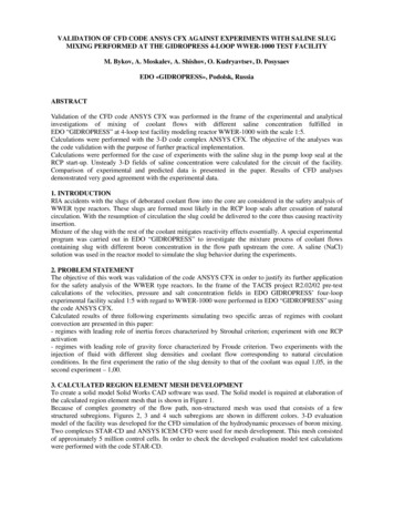
A comparison of the calculation results and experimental data is given in Figures 7 – 9. Figures 7 – 9 providerelative concentration of salt in the place of sensor location. Each Figure shows two curves of salt concentrationvariation in time for the calculated and experimental data respectively. Sensor location is shown in red in thecartogram.5.1 Experiment with the saline slug (initially in the loop seal, volume of 0,12 m3) mixing in the downcomer atRCP start-upThis experiment belongs to regimes for which inertia forces characterized by Strouhal number play the leadingrole. RCP set at Loop 4 is started up and it reaches the nominal flowrate equal to 220 m3/h. Slug volume in Loop 4 is 0,120 m3.It can be seen in Figure 7 the front of salt concentration reaches the core inlet according to the calculated data alittle earlier than according to the data obtained in the experiment. The maximum advance of the calculated front indifferent channels can reach up to 1 second. So the passage of the front and the peak of salt concentration indifferent channels is also shifted by about the same value. From the results of the comparison it is impossible tosingle out exceeding or decrease in the maximum value of salt concentration between the calculated andexperimental data relative to each other. The best agreement of the results is observed in the core centre. Themaximum value of salt concentration is 0,77.It is also seen in Figures 7 that by the end of the studies process at 40 seconds after the experiment has begun, thecalculational and experimental data on salt concentration in different core channels actually coincide. From theabove Figure a good coincidence of the calculational and experimental data is observed that is qualitative in theplace in plan of the model cross-section and that is quantitative in salt concentration.By the results of the analysis it is found that coolant with salt solution goes out of the inlet nozzle of Loop 4 intothe downcomer to the opposite side of reactor model, at this, going downwards. Salt concentration at the core inletfirst appears at the opposite side of the model to the left and to the right relative to the inlet nozzle of Loop 4 .Then it increases directly under the very inlet nozzle of Loop 4. Further on, the front of the increased saltconcentration moves to the core centre and then it gradually decreases.5.2 Experiment with the saline slug (initially in the loop seal, volume of 0,072 m3) mixing in the downcomerat the recover of natural circulation; initial ratio of the slug and the facility coolant densities equals 1,05This experiment belongs to regimes for which gravity forces characterized by Froude number play the leading role.RCP set at Loop 4 is started up and it reaches the nominal flowrate equal to 20 m3/h. Slug volume in Loop 4 is0,072 m3.It can be seen in Figure 8 that the front of salt concentration reaches the core inlet according to the calculated andexperimental data actually simultaneously. The maximum value of salt concentration is 0,34.According to the calculational data the main part of a higher density coolant out of the slug passes the inlet nozzleof Loop 4 and flows down directly under the nozzle itself onto the internal surface of elliptical bottom of reactorvessel model creating a steady “puddle”. "The puddle" gradually smears by a slow main flow of coolant. Becauseof slow flow rate through the core model the flows out of the support tube slots mix up weakly. A star of eight raysin the outlet section of support tubes can be clearly seen. So it is slightly incorrect for the given case to compare theexperimental data of salt concentration obtained from the sensors and the calculational values by the singled outreference volumes.5.3 Experiment with the saline slug (initially in the loop seal, volume of 0,072 m3) mixing in the downcomerat the recover of natural circulation; initial ratio of the slug and the facility coolant densities equals 1,00This experiment belongs to regimes for which gravity forces characterized by Froude number play the leading role.RCP set at Loop 4 is started up and it reaches the nominal flowrate equal to 20 m3/h. Slug volume in Loop 4 is0,072 m3.It can be seen in Figure 9 that the front of salt concentration reaches the core inlet according to the calculated dataabout 5–10 seconds earlier than according to the data obtained in the experiment. The maximum value of saltconcentration reaches 0,49. The best coincidence of the results is observed at the core periphery.
ExperimentANSYS CFXExperimentANSYS CFX28,5 s30 s0.770.690.620.540.460.390.310.230.150.080.0029 s31 s29,5 s31,5 sCC1.00.6ANSYS CFXTestANSYS CFXTest0.80.40.60.40.20.2t / s0.00102030t / s0.004010sensor 12030403040sensor 61CC0.80.8ANSYS CFXTestANSYS CFXTest0.60.60.40.40.20.2t / s0.00102030sensor 1740t / s0.001020sensor 88Fig. 7: Change of concentration at the core inlet
ExperimentANSYS CFXExperimentANSYS CFX64 s78 40.00070 s84 s74 s90 sCC0.40.5ANSYS CFXTestANSYS CFXTest0.40.30.30.20.20.10.10.0020406080100120t / s140100120t / s140100120t / s1400.002040sensor 36080sensor 81CC0.40.4ANSYS CFXTestANSYS CFXTest0.30.30.20.20.10.10.0020406080100sensor 10120t / s1400.0020406080sensor 88Fig. 8: Change of concentration at the core inlet
ExperimentANSYS CFXExperimentANSYS CFX71 s87 90.00076 s94 s80 s100 sCC0.50.5ANSYS CFXTestANSYS CFXTest0.40.40.30.30.20.20.10.10.0020406080100120t / s140100120t / s140100120t / s1400.002040sensor 106080sensor 61CC0.50.5ANSYS CFXTestANSYS or 45120t / s1400.0020406080sensor 67Fig. 9: Change of concentration at the core inlet
The main front of salt concentration passes the core model between 70 and 120 seconds of the experiment. First,the increase in salt concentration is observed at the core periphery opposite to left and to the right of the inletnozzle of Loop 4 and directly under it. It occurs between 71 and 76 seconds and agrees well in place, time andthe values of salt concentrations. Later, between 80 and 87 seconds the maximum values of salt concentration in theexperiment move to the centre of the core inlet and in the calculational analysis they remain in their places. At this,their maximum values coincide. Only after 87 second the maximum calculated values begin moving to the coreinlet. After 100 s of the experiment have passed, the calculated and experimental data again agree well in place,time and the values of salt concentrations.6. CONCLUSIONCFD analyses of the salt concentration distribution in the test facility modeling reactor VVER-1000 was fulfilledwith the complex ANSYS CFX. Numerical simulation of mixing process of coolant flows with various saltconcentrations was performed and parameters of concentration fields in the whole facility were obtained. Results ofCFD analyses demonstrated very good agreement with the experimental data.
model of the facility was developed for the CFD simulation of the hydrodynamic processes of boron mixing. Two complexes STAR-CD and ANSYS ICEM CFD were used for mesh development. This mesh consisted of approximately 5 million control cells. In order to check the developed evaluation model test calculations were performed with the code STAR-CD.