Transcription
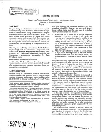
Speeding up SlicingThomas Reps, Susan Horwitz, Mooly Sagiv," ' and Genevieve RosayUniversity of Wisconsin-MadisonABSTRACT1 9 7Program slicing is a fundamental operation for many soft ware engineering tools. Currently, the most efficient algo rithm for interprocedural slicing is one that uses a programrepresentation called the system dependence graph. Thispaper defines a new algorithm for slicing with systemdependence graphs that is asymptotically faster than the pre vious one. A preliminary experimental study indicates thatthe new algorithm is also significantly faster in practice, pro viding roughly a 6-fold speedup on examples of 348 to 757lines.CR Categories and Subject Descriptors: D.2.2 [SoftwareEngineering]; Tools and Techniques - programmer work bench", D.2.6 [Software Engineering]: Programming Envi ronments; D.2.7 [Software Engineering]: Distribution andMaintenance - enhancement, restructuring; E.l [DataStructures] graphsGeneral Terms: Algorithms, PerformanceAdditional Key Words and Phrases: dynamic programming,dynamic transitive closure, flow-sensitive summary informa tion, program debugging, program dependence graph, pro gram slicing, realizable path1. INTRODUCTIONProgram slicing is a fundamental operation for many soft ware engineering tools, including tools for program under standing, debugging, maintenance, testing, and integration[26,13,15,10,6,4]. Slicing was first defined by Mark Weiser,'Work performed while visiting the Datalogisk Institut, University ofCopenhagen, Universitetsparken I, DK-2100 Copenhagen East, Denmark. On leave from IBM Israel, Haifa Research Laboratory.This work was supported in part by a David and Lucile Packard Fellowshipfor Science and Engineering, by the National Science Foundation undergrants CCR-8958530 and CCR-9100424, by the Defense Advanced Re search Projects Agency under ARPA Order No. 8856 (monitored by the Of fice of Naval Research under contract N0(X)14-92-J-1937), by the Air ForceOffice of Scientific Research under grant AFOSR-91-0308, and by a grantfrom Xerox Corporate Research.Authors’ address: Computer Sciences Department; Univ. of Wisconsin;1210 West Dayton Street; Madison, WI 53706; USA.Electronic mail: {reps, horwitz, sagiv, rosay}@cs.wisc.edu.B71204 mwho gave algorithms for computing both intra- and inter procedural slices [26]. However, two aspects of Weiser’sinterprocedural-slicing algorithm can cause it to include“extra” program components in a slice:1.2.A procedure call is treated like a multiple assignmentstatement “vi, V2,.,. 2,., jc ”, where theV/ are the set of variables that might be modified by thecall, and the Xj are the set of variables that might beused by the call. Thus, the value of every v/ after thecall is assumed to depend on the value of every Xjbefore the call. This may lead to an overly conservativeslice (/. ., one that includes extra components) as illus trated in Figure 1.Whenever a procedure P is included in a slice, all callsto P (as well as the computations of the actual parame ters) are included in the slice. An example in which thisproduces an overly conservative slice is given in Figure2.Interprocedural-slicing algorithms that solve the two prob lems illustrated above were given by Horwitz, Reps, andBinkley [14], and by Hwang, Du, and Chou [16]. Hwang,Du, and Chou give no analysis of their algorithm’s complex ity; however, as we show in Appendix A, in the worst casethe time used by their algorithm is exponential in the size ofthe program. By contrast, the Horwitz-Reps-Binkley algo rithm is a polynomial-time algorithm.The Horwitz-Reps-Binkley algorithm (summarized inSection 2) operates on a program representation called thesystem dependence graph (SDG). The algorithm involvestwo steps: first, the SDG is augmented with summary edges,which represent transitive dependences due to procedurecalls; second, one or more slices are computed using theaugmented SDG. The two steps of the algorithm (as well asthe construction of the SDG) require time polynomial in thesize of the program. The cost of the first step—computingsummary edges—dominates the cost of the second step.In this paper we define a new algorithm for interprocedu ral slicing using SDGs that is asymptotically faster than theone given by Horwitz, Reps, and Binkley. In particular, wepresent an improved algorithm for computing summaryedges. This not only leads to a faster interprocedural-slicingalgorithm, but is also important for all other applicationsthat use system dependence graphs augmented with sum mary edges [5,18,7].The new algorithm is presented in Section 3, which alsodiscusses its asymptotic complexity. The complexity of thenew algorithm is compared to that of the Horwitz-RepsBinkley algorithm in Section 4. Section 5 describes someexperimental results that indicate how much better the new
Example programPrecise slice from “output(/)”Slice using Weiser’s algorithmprocedure Mainsum : 0i : 1while / 11 docall A(sum, i)odoutput(5wm)output(/)endprocedure Mainprocedure Mainsum : 0/ : 1while / 11 docall A{sum, i)odoutput(/)endoutput(/)endprocedure A{x, y)X: x yy. y lreturnprocedure A(y)procedure A{x, y)y: y lreturny: y lreturnz : 1while / 11 docall A(z)odFigure 1. An example program, its slice with respect to “output(/)”, and the slice computed using Weiser’s algorithm.Example programprocedure Mainsum : 0z : Iwhile z 11 docall Add(sum, i)call Add(i, 1)odoutput(5zzm)output(z)endPrecise slice from “output(z)”Slice using Weiser’s algorithmprocedure Mainprocedure Mainsum : 0z : Iwhile z 11 docall AddisumJ)can Adda A)odoutput(z)endoutput(z)endprocedure Add{x, y)jc: JC4-yreturnprocedure Addix, y)x: x yreturnprocedure Addix, y)x'.-x yreturnz : 1while z 11 docall Add{i, 1)odFigure 2. An example program, its slice with respect to “output(i)'’, and the slice computed using Weiser’s algorithm.slicing algorithm is than the old one: when implementationsof the two algorithms were used to compute slices for threeexample programs (which ranged in size from 348 to 757lines) the new algorithm exhibited roughly a 6-fold speedup.2. BACKGROUND: INTERPROCEDURAL SLICINGUSING SYSTEM DEPENDENCE GRAPHS2.1. System Dependence GraphsSystem dependence graphs were defined in [14]. Due tospace limitations we will not give a detailed definition here;the important ideas should be clear from the examples. Aprogram’s system dependence graph (SDG) is a collectionof procedure dependence graphs (PDGs): one for each pro cedure. The vertices of a PDG represent the individualstatements and predicates of the procedure. A call statementis represented by a call vertex and a collection of actual-inand actual-out vertices: there is an actual-in vertex for eachactual parameter, and there is an actual-out vertex for eachactual parameter that might be modified during the call.Similarly, procedure entry is represented by an entry vertexand a collection of formal-in and formal-out vertices.(Global variables are treated as “extra” parameters, and thusgive rise to additional actual-in, actual-out, formal-in, andformal-out vertices.) The edges of a PDG represent the con trol and flow dependences among the procedure’s statementsand predicates.* The PDGs are connected together to formthe SDG by call edges (which represent procedure calls, andrun from a call vertex to an entry vertex) and by parameterin and parameter-out edges (which represent parameterpassing, and which run from an actual-in vertex to the corre sponding formal-in vertex, and from a formal-out vertex to‘ As defined in [14], procedure dependence graphs include four kinds ofdependence edges: control, loop-independent flow, loop-carried flow, anddef-order. However, for slicing the distinction between loop-independentand loop-carried flow edges is irrelevant, and def-order edges are not used.Therefore, in this paper we assume that PDGs include only control edgesand a single kind of flow edge.
all corresponding actual-out vertices, respectively).Example. Figure 3 shows the SDG for the program ofFigure 2. DWe wish to point out that SDGs are really a class of pro gram representations. To represent programs in differentprogramming languages one would use different kinds ofPDGs, depending on the features and constructs of the givenlanguage. Although our running example and the experi ments reported in Section 5 use a very simple programminglanguage, the reader should keep in mind that we use theterm “SDG” in this generic sense; in particular, our resultsshould not be thought of as being tied to the restricted lan guage used in our examples. The superiority of the algo rithm given in Section 3 over previous interprocedural slic ing algorithms will almost certainly hold no matter what thefeatures and constructs of the language to which it isapplied. 2.2. Interprocedural SlicingPDG: to compute the slice with respect to PDG vertex v,find all PDG vertices from which there is a path to v alongcontrol and/or flow edges [22]. Interpvoceduved slices canalso be obtained by solving a reachability problem on theSDG; however, the slices obtained using this approach willinclude the same “extra” components as illustrated in col umn 3 of Figure 2. This is because not all paths in the SDGcorrespond to possible execution paths. For example, thereis a path in the SDG shown in Figure 3 from the vertex ofprocedure Main labeled ''sum: 0” to the vertex of Mainlabeled “output(/).” However, this path corresponds to an“execution” in which procedure Add is called from the firstcall site in Main, but returns to the second call site in Main,which is not a legal call/return sequence. The final value ofi in Main is independent of the value of sum, and so the ver tex labeled "sum:-O'" should not be included in the slicewith respect to the vertex labeled “output(i)”.Instead of considering all paths in the SDG, the computa tion of a slice must consider only realizable paths: paths thatreflect the fact that when a procedure call finishes, executionOttenstein and Ottenstein showed that m/raprocedural slicescan be obtained by solving a reachability problem on theEdge Keycontrol edge- flow edgecall,parameter-in, orparameter-outedgeFigure 3. The SDG for the program of Figure 2.“The issue of how to create appropriate PDGs/SDGs is orthogonal to theissue of how to slice them. Previous work has investigated how to builddependence graphs for the features and constructs found in real-world pro gramming languages. For example, previous work has addressed arrays[3,27,21,11,23,24], reference parameters [14], pointers [20,12,8], and nonstructured control flow [2,9,1].output
returns to the site of the most recently executed call. sum : 0Definition (realizable paths). Let each call vertex in SDGG be given a unique index from 1 to k. For each call site C/,label the outgoing parameter-in edges and the incomingparameter-out edges with the symbols “(/” and “)/”» respec tively; label the outgoing call edge with “(/” A path in G is a same level realizable path iff thesequence of symbols labeling the parameter-in, parameterout, and call edges in the path is a string in the language ofbalanced parentheses generated from nonterminal matchedby the following context-free grammar:matchedmatchedmatched ),for 1 / /:1 sA path in C is a realizable path iff the sequence of sym bols labeling the parameter-in, parameter-out, and call edgesin the path is a string in the language generated from nonter minal realizable by the following context-free grammar(where matched is as defined above):realizableIrealizable (, matchedmatchedfov\ i k Example. In Figure 3, the pathXin : sumx :x ,nf : Xsum : is a (same-level) realizable path, while the pathsum : 0— Xifj : sum -» x : Xi — jc : jc -t- y: X — /: Xoutoutput(/)is not. An interprocedural-slicing algorithm is precise up to real izable paths if, for a given vertex v, it determines the set ofvertices that lie on some realizable path from the entry ver tex of the main procedure to v. To achieve this precision,the Horwitz-Reps-Binkley algorithm first augments theSDG with summary edges, A summary edge is added fromactual-in vertex v (representing the value of actual parame ter X before the call) to actual-out vertex w (representing thevalue of actual parameter y after the call) whenever there isa same-level realizable path from v to w. The summaryedge represents the fact that the value of y after the callmight depend on the value of x before the call. Note that asummary edge cannot be computed simply by determiningwhether there is a path in the SDG from v to w {e.g., by tak ing the transitive closure of the SDG’s edges). Thatapproach would be imprecise for the same reason that tran sitive closure leads to imprecise interprocedural slicing,Figure 4. The SDG of Figure 3, augmented with summary edges and sliced with respect to “output{/)”.similar goal of considering only paths that correspond to legalcall/retum sequences arises in the context of interprocedural dataflowanalysis [25,19]. Several different terms have been used for these paths,including valid paths, feasible paths, and realizable paths.jc : jc y— output(5Mm)
namely that not all paths in the SDG are realizable paths.After adding summary edges, the Horwitz-Reps-Binkleyslicing algorithm uses two passes over the augmented SDG;each pass traverses only certain kinds of edges. To slice anSDG with respect to vertex v, the traversal in Pass 1 startsfrom V and goes backwards (from target to source) alongflow edges, control edges, call edges, summary edges, andparameter-in edges, but not along parameter-out edges. Thetraversal in Pass 2 starts from all actual-out vertices reachedin Pass 1 and goes backwards along flow edges, controledges, summary edges, and parameter-out edges, but notalong call or parameter-in edges. The result of an interpro cedural slice consists of the set of vertices encountered dur ing Pass 1 and Pass 2, and the edges induced by thosevertices." Example. Figure 4 gives the SDG of Figure 3 augmentedwith summary edges, and shows the vertices and edges tra versed during the two passes when slicing with respect tothe vertex labeled “output(/).” 3. AN IMPROVED ALGORITHM FOR COMPUTINGSUMMARY EDGESThis section contains the main result of the paper: a newalgorithm for computing summary edges that is asymptoti cally faster than the one defined by Horwitz, Reps, andBinkley. (We will henceforth refer to the latter as the HRB summary algorithm.)The new algorithm for computing summary edges isgiven in Figure 5 as function Computes ummaryEdges,(ComputesummaryEdges uses several auxiliary accessfunctions: function Proc returns the procedure that containsthe given SDG vertex; function Callers returns the set ofprocedures that call the given one; function CorrespondingActualln (and CorrespondingActualOut) returns the actualin (or actual-out) vertex associated with the given call sitethat corresponds to the given formal-in (or formal-out) ver tex.) Figure 6 illustrates schematically the key steps of thealgorithm. The basic idea is to find, for every procedure P,ail same-level realizable paths that end at one of P’s formalout vertices. Those paths that start from one of P’s formal in vertices induce summary edges between the correspond ing actual-in and actual-out vertices at all call sites that rep resent calls to P. (For example, if the algorithm wereapplied to the SDG shown in Figure 3, a path would befound from the formal-in vertex of procedure Add labeled to the formal-out vertex labeled: jc”.This path would induce the summary edges from to ''sum : and from "Xin\ r to"i : in Main, as shown in Figure 4.)“ The augmented SDG can also be used to compute a forward (interproce dural) slice using two edge-traversal passes, where each pass traverses on ly certain kinds of edges; however, in a forward slice edges are traversedfrom source to target. The first pass of a forward slice ignores parameterin and call edges; the second pass ignores parameter-out edges.In the algorithm, same-level realizable paths are repre sented by “path edges”, the edges that are inserted into theset called PathEdge. The algorithm starts by “asserting”that there is a same-level realizable path from every formalout vertex to itself; these path edges are inserted intoPathEdge, and also placed on the worklist. Then the algo rithm finds new path edges by repeatedly choosing an edgefrom the worklist and extending (backwards) the path that itrepresents as appropriate depending on the type of thesource vertex. This is illustrated in Figure 6. When a pathedge is processed whose source is a formal-in vertex, thecorresponding summary edges are inserted into the Summa ry Edge set (lines [16]-[19]). These new summary edgesmay in turn induce new path edges: if there is a summaryedge x y, then there is a same-level realizable pathX —y a for every formal-out vertex a such that there is asame-level realizable path y—y a. Therefore, procedurePropagate is called with all appropriate x—edges (lines[20]-[22]).The cost of the algorithm can be expressed in terms of thefollowing parameters:pSites pSitesTotalSitesEParamsThe number of procedures in the pro gram.The number of call sites in procedure p.The maximum number of call sites inany procedure.The total number of call sites in the pro gram. (This is bounded by P x Sites.)The maximum number of control andflow edges in any procedure’s PDG.The maximum number of formal-in ver tices in any procedure’s PDG.The algorithm finds all same-level realizable paths that endat a formal-out vertex vv. A new path jc —y w is found byextending (backwards) a previously discovered path v —vv(taken from the worklist) along the edge x — v. Becausevertex .x can have out-degree greater than one, the same pathcan be discovered more than once (but it will only be put onthe worklist once, due to the test in Propagate).In the worst case, the algorithm will “extend a path”along every PDG edge (lines [27]-[29]) and every summaryedge (lines [11]”[13] and [20]-[22]) once for each formalout vertex. Thus, the cost of computing summary edges fora single procedure is equal to the number of formal-out ver tices (bounded by Params) times the number of PDG andsummary edges in that procedure. In the worst case, there isa summary edge from every actual-in vertex to every actualout vertex associated with the same call site. Therefore, thenumber of summary edges in procedure p is bounded by0(SiteSp X Params ), and the cost of computing summaryedgesforoneprocedureisboundedby0(Params x ( " {Sites x Params ))), which is equal to0{{Params x E) {Sites x Params )). Summing overall procedures in the program, the total cost of the algorithmis bounded by
function ComputeSummaryEdges(G: SDG) returns set of edgesdeclare PathEdge, SummaryEdge, WorkList: set of edges[1]procedure Propagate( : edge)beginif PathEdge then insert e into PathEdge; insert e into WorkList fiend[2][3][4][5][6]beginPathEdge0; SummaryEdge : 0; WorkList : 0for each w e FormalOutVertices{G)insert (ww) into PathEdgeinsert (w — vv;) into WorkListod[7][8][9]while WorkList 0 doselect and remove an edge v — w from WorkListswitch V[10][11][ 12][13][14]case V e ActualOutVertices(G):for each x such that x— ve {SummaryEdge u ControlEdgesiG)) doPropagate(jc — w)odend case[15][16][17][18][ 19][20][21][22][23][24][25]case v FormallnVertices{G):for each c Callers{Proc{w)) dolet jc CorrespondingActuaIIn(c, v)y CorrespondingActualOutCc, w) ininsert x — y into SummaryEdgefor each a such that y — a e PathEdge doPropagate( — odend letodend case[26][27][28][29][30]default:for each x such that jc — v g {FlowEdges{G) u ControlEdgesiG)) doPropagate(jc — w)odend case[31 ][32][33]end switchodretum(SummaryEdge)endFigure 5. Function ComputeSummaryEdges computes and returns the set of summary edges for the given system dependence graph G(See also Figure 6.)0{{PXParams x ) {TotalSites x Params )).4. COMPARISON WITH PREVIOUS WORKThe cost of interprocedural slicing using the algorithm ofHorwitz, Reps, and Binkley is dominated by the cost ofcomputing summary edges via the HRB-summary algorithm(see [14]):0{{TotalSites x E x Params) (TotalSites x Sites x Params )).The main result of this paper is a new algorithm for comput ing summary edges whose cost is bounded by0{(P X E X Params) (TotalSites x Params )),Under the reasonable assumption that the total number ofcall sites in a program is much greater than the number ofprocedures, each term of the cost of the new algorithm isasymptotically smaller than the corresponding term of thecost of the HRB-summary algorithm. Furthermore, becausethere is a family of examples on which the HRB-summaryalgorithm actually performsQ((TotalSites x E x Params) (TotalSites x Sites x Params ))steps, the new algorithm is asymptotically faster.There are two main differences in the approaches takenby the two algorithms that lead to the differences in their
costs:1. The HRB-summary algorithm first creates a “com pressed” form of the SDG that contains only formal-in,formal-out, actual-in, and actual-out vertices. The edgesof the compressed graph represent (intraprocedural)paths in the original graph. The cost of compressing theSDG is 0{TotalSites x E x Params), the first term inthe cost given above. The new algorithm uses theuncompressed SDG, so there is no compression cost.2. After compressing the SDG, the HRB-summary algo rithm repeatedly finds and installs summary edges, thencloses the edge set of the PDG. These “install-andclose” steps are similar to the “extend-a-path” steps thatare performed by the new algorithm. The difference isthat the “close” step of the HRB-summary algorithmessentially replaces a 3-part path of the form“path:edge:path” with a single path edge, while the newalgorithm replaces a 2-part path of the form “edge:path”with a single path edge. The latter approach is a secondreason for the superiority of the new algorithm. Thetotal cost of the series of “install-and-close” steps per formedbytheHRB-summaryalgorithmis0{TotalSites x Sites x Params" ), the second term inthe cost given above. This term is likely to be the domi nant term in practice, and it is worse (by a factor ofSites X Params) than the second term in the new algo rithm’s cost.To summarize: Both the cost of the HRB-summary algo rithm and the cost of the new algorithm contain two terms.In the case of the former, the first term represents the cost ofcompression, and the second term represents the cost offinding summary edges using the compressed graph. In thecase of the latter, both terms represent the cost of findingsummary edges using the uncompressed graph. The cost ofthe new algorithm is asymptotically better than the cost ofthe HRB-summary algorithm.5. EXPERIMENTAL RESULTSThis section describes the results of a preliminary perfor mance study we carried out to measure how much fasterinterprocedural slicing is when function ComputeSummaryEdges is used in place of the HRB-summary algorithm.The slicing algorithms were implemented in C and tested ona Sun SPARCstation 10 Model 30 with 32 MB of RAM.Tests were carried out for three example programs (writtenin a small language that includes scalar variables, array vari ables, assignment statements, conditional statements, outputstatements, while loops, for loops, and procedures withvalue-result parameter passing): recdes is a recursivedescent parser for lists of assignment statements; calc is asimple arithmetic calculator; znd format is a text-formattingprogram taken from Kernighan and Plauger’s book on soft ware tools [17]. The following table gives some statisticsabout the SDGs of the three test programs:SDG statisticsLinesVer ControlPSites TotalSitesProg. oftices 1465144332761524531326206070108 EParams25540959781223The comparison in Section 4 of the asymptotic worst-caserunning time of the HRB-summary algorithm with that ofthe new algorithm suggests that the new algorithm shouldlead to a significantly better slicing algorithm. However,formulas for asymptotic worst-case running time may not begood predictors of actual performance. For example, theformula for the running time of ComputeSummaryEdgeswas derived under the (worst-case) assumptions that there isa summary edge from every actual-in vertex to every actualout vertex associated with the same call site, and that everycall site has the same number of actual-in and actual-outvertices—both of which are bounded by Params, Thisyields 0{TotalSites x Params ) as the bound on the totalnumber of summary edges. As shown in the followingtable, this overestimates the actual number of summaryedges by one to two orders of magnitude:ExamplerecdescalcformatTotalSites x Params Actual number ofsummary edges38401008057132157227413Thus, although asymptotic worst-case analysis may be help ful in guiding algorithm design, tests are clearly needed todetermine how well a slicing algorithm performs in practice.For our study, we implemented three different slicingalgorithms: (A) the Horwitz-Reps-Binkley slicing algo rithm, (B) the slicing algorithm with the improved methodfor computing summary edges from Section 3, and (C) analgorithm that is essentially the “dual” of Algorithm B.Algorithm C is just like Algorithm B, except that the com putation of summary edges involves finding all same-levelrealizable paths/ram formal-in vertices (rather than to formal-out vertices), and paths are extended forwards ratherthan backwards.The table shown in Figure 7 gives statistics about the per formance of the three algorithms for a representative slice ofeach of the three programs. In each case, the reported run ning time is the average of five executions. (The quantity“Time to slice” is “user cpu-time system cpu-time”.) Thetime for the final step of computing slices—the two-passtraversal of the augmented SDG—is not shown as a separateentry in the table; this step is a relatively small portion of thetime to slice: .03-.04 seconds (of total cpu-time) for bothrecdes and calc; .20-.23 seconds for format.As shown in columns 6 and 8 of the above table. Algo rithms B and C are clearly superior to Algorithm A, exhibit ing 4.8-fold to 6.5-fold speedup. Algorithm B appears to be
Lines [16]-[191KEY control or flow edgepath edge(possibly new) path edgesummary edgenew summary edgeparameter-in orparameter-out edgeFigure 6. The above four diagrams show how the algorithm of Figure 5 extends same-level realizable paths, and installs summary edges.Vertices in sliceExamplerecdescalcformatHRB slicingalgorithmNumberPercentof totalTime to slice(seconds)413484132749%58%72%2.08 0,043.06 0.056.64-H 0.12Algorithm BSummary edges computedby the algorithm ofSection 3Time to sliceSpeedup(seconds)(over HRB)0.35 0.040.46 0.030.98 0.125.46.36.1Algorithm CSummary edges computedby the dual of thealgorithm of Section 3Speedup(over HRB)0.45 0.031.09 0.164.86.55.4Figure 7. Performance of the three algorithms for a representative slice of each of the three example programs.marginally better than Algorithm C. We believe that this isbecause procedures have fewer formal-out vertices than for mal-in vertices.Because the bound derived for the series of “install-andclose” steps of Algorithms B and C is better than the boundfor the HRB-summary algorithm by a factor ofSites X Params, the speedup factor may be greater onlarger programs. As a preliminary test of this hypothesis,we gathered some statistics on versions of the above pro grams in which the number of parameters was artificiallyinflated (by adding additional global variables). On theseexamples, Algorithm C exhibited 10-fold speedup over theHorwitz-Reps-Binkley slicing algorithm, and Algorithm Bexhibited 13-fold to 23-fold speedup.In summary: the conclusion that the algorithm presentedin this paper is significantly better than the Horwitz-RepsBinkley interprocedural-slicing algorithm is supported bothby comparison of asymptotic worst-case running times (seeSection 4) and preliminary experimental results.APPENDIX A; Demonstration that the Algorithm ofHwang, Du, and Chou is ExponentialThe Hwang-Du-Chou algorithm constructs a sequence ofslices of the program—where each slice in the sequenceessentially permits one additional level of recursion—until afixed point is reached {ie,, until no further elements areincluded in a slice). In essence, to compute a slice withrespect to a point in procedure P, it is as if the algorithmperforms the following sequence of steps:1.Replace each call in procedure P with the body of thecalled procedure.2. Compute the slice using the new version of P (andassume that there are no flow dependences across unex panded calls).
3.Repeat steps 1 and 2 until no new vertices are includedin the slice, (For the purposes of determining whether anew vertex is included in the slice, each vertex instancein the expanded program is identified with its “originat ing vertex” in the original, multi-procedure program.)In fact, no actual in-line expansions are performed; insteadthey are simulated using a stack. On theslice of thesequence, there is a bound of k on the depth of the stack.Because the stack is used to keep track of the calling contextof a called procedure, only realizable paths are considered.In this appendix, we present a family of examples onwhich the Hwang-Du-Chou algorithm takes exponentialtime. In order to simplify the presentation of this family ofprograms, we will streamline the diagrams of the SDGs weuse by including only vertices related to procedure calls(enter, formal-in, formal-out, call, actual-in, and actual-outvertices) and the intraprocedural transitive dependencesamong them. (This streamlining does not affect our argu ment, and showing complete SDGs would make our dia grams unreadable.)Theorem. There is a family of programs on which theHwang-Du-Chou algorithm uses time exponential in the sizeof the program.Proof. We construct
Speeding up Slicing Thomas Reps, Susan Horwitz, Mooly Sagiv," ' and Genevieve Rosay University of Wisconsin-Madison 1 9 7 ABSTRACT Program slicing is a fundamental operation for many soft