WIXLIB

Lawonn et al. / Streamlines for Illustrative Real-Time Renderingthe use of transparancy and texturing techniques to illustrate vector fields. Buchin et al. [BW03] present a hatchingscheme which can interactively change the stroke style. Zander et al. [ZISS04] use streamlines instead of textures to generate hatching lines based on curvature information. Gerl etal. [GI13] present a way to intuitively interact with the hatching illustration based on hand-drawn examples. They used ascanned-in hatching picture as input and machine learningmethods to learn a model of the drawing style. A combination of different rendering techniques for medical applications was presented by Tietjen et al. [TIP05].In summary, the available feature line methods are not sufficient to depict arbitrary shapes, especially in the domainof anatomical structures. They highlight features, but localshape properties, which relate to curvature changes, are often not satisfyingly represented. The latter is resolved byhatching methods, which have the drawbacks of being dependent on texturing or drawing too many hatching patterns.Thus, real-time performance can not always be guaranteedin combination with high visual quality.3.2. Feature Regions3. Method ConFIS is based on streamlines to illustrate the surfacemodel. For this reason, we will first describe the regionswhere we want to seed the streamlines. Second, we explainhow to calculate streamlines. For this, we divide this sectionin three parts:1. Contour margin: We offer a definition for the contour.Furthermore, we explain the term contour margin.2. Feature regions: We provide a curvature-based definition for a feature region.3. Streamlines: We explain how to determine explicitstreamlines.3.1. Contour MarginDefinition 3.1 (Contour) The contour is defined as the lociof points where the surface normal and the view vector aremutually perpendicular (ϑ 90 ).For an extended overview about contours we refer to Isenberg et al. [IFH 03]. We highlight the common edge of twoadjacent triangles if the signs of the dot products between theoriented face normals and the view vector change. Besidesthe contour line, we also draw streamlines at contour triangles. As we want to provide frame-coherent interaction, weseed streamlines at triangles which lie inside a contour margin. The contour margin is defined by the curvature-basedmethod of Kindlmann et al. [KWTM03]. Triangles are included in the contour margin if the dot product of the normal and the view vector is less than T κv (2 T κv ). Here, κvdenotes the normal curvature in direction of the view vectorand T denotes the thickness. This method provides a homgeneous contour margin in image space. Additionally, theopacity of the streamlines changes depending on the lengthto provide a convenient fade-off during the interaction.c 2013 The Author(s)c 2013 The Eurographics Association and Blackwell Publishing Ltd.Definition 3.2 (Maxima and minima on a scalar field) Continuous Case: Maxima and minima can occur wherethe gradient of the scalar field vanishes. Discrete Case: We determine the gradient of the scalarfield for each vertex of a triangle. The three dot products between the gradients are calculated. A maximumor a minimum occurs if two dot products are negative toidentify zero-crossings.We seed a feature streamline at a triangle t if the followingproperties for the mean curvature field (MCF) are fulfilled:i. The MCF has a maximum or a minimum at t.ii. The MCF at t exceeds a user-specified threshold.3.3. StreamlinesStreamlines are seeded at every contour triangle and withina defined margin around the contour. Thus, the following issues have to be solved:Choose a suitable vector field.Select an appropriate starting point.Estimate the maximum streamline length.Calculate the streamline.Use an adaptive step size for the streamlines.The vector field for streamline calculation: We choose asuitable curvature-based vector field for streamline calculation. In order to compute curvatures on a discrete triangle mesh, the algorithm from Rusinkiewicz [Rus04] is used,since it yields accurate and robust results even on irregularly tessellated surfaces. The curvature tensor of each triangle is determined by using finite differences of the vertexnormals in direction of the edges. The vertex normals are obtained by averaging the area-weighted normals over adjacentfaces. Afterwards, we compute the curvature tensor for every vertex by averaging the curvature tensors of the trianglesadjacent to each vertex. The eigenvectors and eigenvaluesprovide the principal curvatures (PCs) and curvature directions (PCDs). At umbilic vertices, we set the PCDs to thezero vector and exclude the streamlines from seeding. Weassign four vectors at the vertices and the triangle – namelytwo PCDs, each with two possible signs. For each triangle,only t1 is used where t1 is the PCD which corresponds tothe maximum PC. We compare t1 of each triangle with thefour vectors of their adjacent vertices. We determine the dotproduct between t1 and the four vectors of the first vertex.We select the vector which corresponds to the largest dotproduct. The resulting vector belongs to the final vector fieldto ensure that is smooth. We repeat this with the other twovertices, determine the dot products and use the vector whichmaximizes them. By doing so, we obtain a triple (e1 , e2 , e3 )of vectors for each triangle. We use the triple (e1 , e2 , e3 ) and( e1 , e2 , e3 ) to get two vector fields for each triangle bybarycentric interpolation. With these two final vector fields,

Lawonn et al. / Streamlines for Illustrative Real-Time Renderingstreamline c(t) fulfills the following condition: c(t) e2 e1 e3 e1 c(t) e1 . t {z}(2)CAvxpuFigure 2: Every point p in the triangle can be representedby the basis (u, v) with coefficients (α, β), α, β 0 and α β 1. The corresponding resulting vector e(p) can be obtainedwith the point p (α, β) by: e(p) (e2 e1 e3 e1 ) · p e1 .we can generate two different streamlines for each triangle.Streamline starting points: Every streamline starts at thebarycenter of the contour triangle. Furthermore, we are alsoseeding streamlines at the barycenter of adjacent triangleswithin the contour margin. As we want to achieve frame coherence, we have to start the streamlines at consistent startpositions. We also generated streamlines at different randomly chosen start positions, but we could not see any visualdifference. Thus, we stay at the choice of the barycenter asthe start position for the streamlines.Streamline length: We employ the principal curvatures todetermine the length of the streamline. Every triangle obtains a minimum and maximum curvature κ1 , κ2 . The lengthL of a streamline is calculated by:L π.3 · max{ κ1 , κ2 }(1)We want the streamline to have a length of one third of thethe half perimeter of the osculating circle: 31 πr. If the streamline length L exceeds a user-defined threshold Lmax , we setL Lmax . We suggest the median value of all calculatedlengths per vertex for the streamline length threshold Lmax .Calculation of the streamline: Some authors use implicit orexplicit iterative methods for the approximation of ordinarydifferential equations, e.g., [ZISS04]. Nielson et al. [NJ99]determined explicit streamlines over tetrahedral domains.Furthermore, they gave the solution for streamlines over triangle domains. We derive the explicit streamline solution foreach triangle and describe this process in detail. Given a triangle t (p1 , p2 , p3 ) with associated PCDs (e1 , e2 , e3 ), theassociated (non-normalized and non-orthogonal) basis (u, v)is built by: u p2 p1 and v p3 p1 . Every position p andthe associated vector e(p) in the interior of the triangle can becalculated by the basis (u, v), see Figure 2. The parametrizedSuch an inhomogeneous ODE (iODE) c0 Ac e1 is solvedby the method of separation of constants [Pag97, Har64].First, we solve the homogeneous ODE (hODE) c̃0 Ac̃. Afterwards, we determine the missing factor for the inhomogeneous part e1 . The solution of c̃0 Ac̃ is a linear combinaPAk ·tktion of a fundamental solution: c̃(t) exp(A · t) k 0 k! .In practice, we decompose the Matrix A in a Jordan-form:A DJD 1 . Then we obtain c̃(t) D · exp(J · t) · D 1 . Asthe inverse is not necessary for a fundamental solution system, we get c̃(t) D · exp(J · t) as a fundamental system.The solution leads us to the general solution of the ODE:c(t) c p (t) c̃(t). We claim c p (t) c̃(t) · f (t) with an arbitrary 2D differentiable function f (t) to determine a particularsolution c p (t) for the iODE. The derivative of c p (t) yields: c p (t) A · c(t) c̃(t) · f 0 (t).(3) tComparing Equation 2 with Equation 3 leads to: c̃(t) · f 0 (t) e1 . Finally, the particular solution has the form:"Z t#c p (t) D · exp(J · t) ·exp( J · x) dx · D 1 · e1 C. (4)t0For simplicity, we write c p (t) as an indefinite integral andleave out the constant C. Furthermore, we write"Z#A(t) B D · exp(J · t) ·exp( J · t) dt · D 1 .(5)We have got the final fundamental solution for the ODE. Forthe specific solution we need the parameters x1 , x2 R forthe hODE. With the restriction c(0) p, we obtain the condition: p A(0) · e1 D · xx12 . Solving this equation with respect to x1 , x2 yields:!x1 D 1 · (p A(0) · e1 ) .(6)x2Again, we refer to the appendix for a comprehensive form ofx1 , x2 . Finally, we get the explicit streamline representationstarting at position p with 4 and 6:!x1c(t) c p (t) c̃(t) ·(7)x2 A(t) · e1 D · exp(J · t) · D 1 · (p A(0) · e1 ) .(8)The streamline representation depends on the terms exp(J · t)and A(t), which can be simplified, see Sec. 8. Within thetriangle, streamlines have the following properties: c(t) x 0, c(t)y 0, and c(t) x c(t)y 1. Violating one conditionleads to an intersection point of the streamline with one ofthe edges. Thus, we get the adjacent triangle of the edge. Wecan determine the underlying vector field of the new triangle according to Section 3 (The vector field for streamlinecalculation). Instead of using the triangle PCD as referencec 2013 The Author(s)c 2013 The Eurographics Association and Blackwell Publishing Ltd.

Lawonn et al. / Streamlines for Illustrative Real-Time RenderingTriangleDataRendering LoopDetermineContour torageBufferDetect FeaturesTransformFeedbackTransformFeedbackDraw StreamlinesFigure 3: The scheme of ConFIS which is divided in two parts: the preprocessing and the rendering part.direction, we employ the streamline direction vector.Adaptive step size: For streamline propagation we use anadaptive step size. Whenever the length of a streamline segment exceeds the inradius of the triangle, we halve the stepsize. This ensures that the streamline will not immediatelyleave the triangle in most cases. Furthermore, the visual results of the streamlines seem to be smooth, although we donot have to calculate too much line segments in a triangle.3.4. Advantage of explicit streamline calculationFirst of all, determining the explicit streamline exhibits alower error than iterative methods for the approximation ofODEs. Explicit streamlines do only produce an error whenapproximating the intersection point of one edge of the triangle with the streamline. Another advantage of explicitstreamlines is the converging propagation behavior towardssingularities. The explicit streamline will converge into thispoint. An iterative streamline can oscillate around the singularity. Moreover, iterative methods are based on a sequenceof points. Thus, one point can only be approximated by usingthe previously calculated ones. In contrast, explicit streamlines can be calculated in parallel without knowing the previous points.4. Algorithm and GPU ImplementationThe algorithm for ConFIS on the mesh M is as follows:1. (Optional) Subdivide and smooth M.2. Compute the PCDs and the corresponding PCs.3. Determine feature regions of M.4. Compute two streamlines for all triangles.5. Compute the contour and contour margin.6. Draw the contour and feature streamlines.The algorithm is divided in two different parts. The first part(1.-4.) consists of the preprocessing steps and the second part(5.-6.) is executed during runtime (see Fig. 3). As shown earlier, the generation of a streamline for an arbitrary trianglerequires to traverse M iteratively from one triangle to thenext. For achieving a fast rendering, several APIs, such asCUDA, OpenCL, or DirectCompute are available. We choseto perform all computations with the OpenGL shader framework to be independent of graphics card vendors and toc 2013 The Author(s)c 2013 The Eurographics Association and Blackwell Publishing Ltd.reduce any overhead by additional APIs. The shader concept is ideally suited for per-vertex and per-triangle operations, which are required by our streamline method. OpenGLshaders do natively not provide neighborhood information,such as the 1-ring of each vertex. Thus, we employ a datastructure similar to the one which has been presented in[MKL 12]. Topological information, such as the locationof neighboring vertices, is made available via vertex (VBO)and texture buffer objects (TBO). With this, we can seed andcontinue tracking a streamline at each triangle for an arbitrary number of triangles.4.1. PreprocessingFirst, we generate two streamlines at the barycenterfor each triangle with given length (recall Sec. 3).These processing steps are entirely executed on theGPU via OpenGL shaders. Such a streamline buffercontains #Triangles #LineSegments 2 elements. Forwriting the streamline vertices to this buffer, we useshader storage buffer objects. Thus, the OpenGL extensionARB SHADER STORAGE BUFFER OBJECT, which ispart of the OpenGL core since version 4.3, is required. Withthis, each triangle is able to write the vertices belonging toeach of its two streamlines into the streamline buffer. Additionally, the preprocessing step allows for a detection ofthose triangles which shall later generate a feature streamline based on the curvature criterion (see Sec. 3.2). Until thispoint, nothing has been drawn – but all the streamlines havebeen precomputed for later rendering.4.2. Rendering loopDuring runtime, the steps 5 and 6 are executed. Using geometry shaders, we can determine the object contour anda defined contour margin. Thus, we could access the previously generated streamline buffer and start drawing contour and feature streamlines. Unfortunately, this yields a badload balancing, since we seed streamlines only at comparably few triangles. Most geometry shader invocations wouldnot perform any streamline processing. In the worst case, allthreads in one thread group have to wait until all streamlinegeneration-threads finish – even if only one thread is generating a streamline.

Lawonn et al. / Streamlines for Illustrative Real-Time Rendering(a) Ribs(b) Inside view of the pulmonary arteryFigure 4: The ConFIS method with two anatomical surface models.Thus, we split the rendering stage into two render passes.At first, all triangles, which shall draw a contour streamline (recall Sec. 3.3), are identified and marked. For eachof these triangles and those which have been marked duringpreprocessing for seeding feature streamlines, we store triangle information (e.g., vertex IDs) using OpenGL’s transform feedback mechanism. In the seconds pass, renderingis performed only for the marked triangles. As a result, theGPU processes only triangles which contribute to streamlinerendering. Each of these triangles can access the completestreamline buffer via TBOs. The opacity of each streamlineis reduced with increasing length.in different order. They had the possibility to explore themodel interactively and gain a 3D impression.2. The second task was to adjust the specific parameters ofthe illustration methods to obtain a subjectively satisfyingand informative result. During this, we noted the participants’ spoken comments and the parameter sets they weresatisfied with.3. The third part of the evaluation consisted of a visual comparison and a qualitative assessment between the feature line methods. Based on the recorded parameter sets,each participant should assess which method is considered more appropriate to express surface features andwhich limitations have been observed.5. EvaluationAneurysm 1 model: The participants mentioned that thegenerated lines by the feature line methods were not appropriate to gain a comprehensive spatial impression. Most ofthe generated lines were considered distracting. On the otherhand, these methods depicted parts of the bifurcation well.All participants agreed that the hatching method generates areasonable 3D impression. For HQ, the evenly spread linescan not depict important features, e.g., the border betweenthe vessel and aneurysm sac. Furthermore, several participants criticized the low performance of the HQ implementation ( 13 fps). ConFIS fulfilled the demands to illustraterelevant features and to convey an appropriate 3D impression. All participants chose ConFIS as their preferred linedrawing technique.We performed a qualitative evaluation for the five line drawing techniques: suggestive contour (SC), apparent ridges(AR), photic extremum lines (PEL, according to Zhang etal. [ZHX 11]), high quality hatching (HQ), and ConFIS. Thegoal was to assess their capabilities for expressing relevantsurface characteristics. We wanted to figure out which ofthe line drawing methods yields the most expressive resultfor the participants. The evaluation was conducted with twophysicians and three researchers with background in medicalvisualization. Four representative surface models were chosen: ribs (Fig. 4(a)), aneurysm 1 (Fig. 5, middle row), trachea (Fig. 5, bottom row), and femur (Fig. 6(d)). The models are derived from segmenting medical image data and preprocessed to ensure an appropriate and homogeneous degreeof tessellation. For all compared methods, we employed theoriginal implementations by the corresponding authors. Theevaluation was conducted in three steps:1. Each participant was shown the shaded surface modelsTrachea model: The inner view of the trachea has twofeatures: the elongated structure and the bifurcation, wherethe carina tracheae splits into both branches. The participants confirmed that the feature line methods can depict theelongated structures but fail to enhance the carina tracheae.Apart from that, they explained that the hatching method asc 2013 The Author(s)c 2013 The Eurographics Association and Blackwell Publishing Ltd.

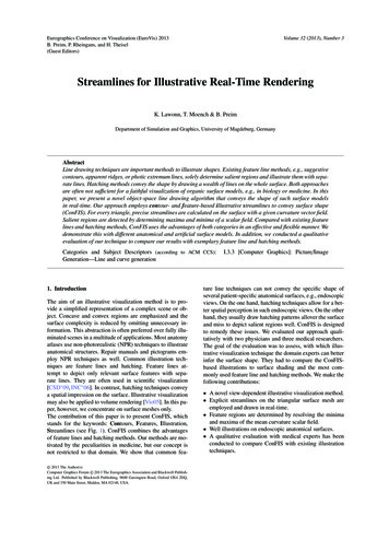
Lawonn et al. / Streamlines for Illustrative Real-Time RenderingSCARPELHQConFISFigure 5: Different surface models displayed with suggestive contour (SC), apparent ridges (AR), photic extremum lines (PEL),high quality hatching (HQ), and ConFIS. The models are from top to bottom: hyperthing, aneurysm 1, and endoscopic view ofa tracheawell as ConFIS depict both properties well. One participantfound some streamlines slightly disturbing and unnecessaryto gain a spatial impression. The hatching method could nothighlight the bifurcation features. In contrast, it looked likea planar transition from one bronchus to the other. Finally,all participants preferred the ConFIS method.Ribs model: The ribs model was chosen to evaluate the3D feeling of the mesh even if the surface has a lot of structures. The participants get a reasonable 3D impression byall line drawing methods. Some participants mentioned thatthere are only small differences between the feature linemethods. One participant explained that the impression ofthe model is appropriate during the interaction but seeingonly a screenshot would confuse. The participant could notset the ribs apart from the gaps. Furthermore, some lineswhich are produced by feature line methods are distractingand the hatching method can not illustrate the dents. ConFISillustrates all ribs well and the participants can distinguishthe ribs from the gaps and all dents are depicted as well.Femur model: Some of the participants found fault withthe view-dependent feature illustrations. The feature linemethods only show some dents first if the camera position ischosen well. Again, two participants criticized the missingdetails using the hatching method. Some dents are missingc 2013 The Author(s)c 2013 The Eurographics Association and Blackwell Publishing Ltd.and without interactive exploration some important regionsare missed. Those regions have been highlighted with ConFIS, which was again preferred.The results of our evaluation can be summarized as follows: Current line drawing techniques achieve satisfying resultsonly if the models exhibit a smooth and regularly tessellated surface. The clutter of surfaces derived from measured image data,such as noise and staircase artifacts, are usually emphasized. For some cases, line drawing methods are not able to depict relevant features. The ConFIS method was the most expressive technique inour comparison.However, the informal study does not allow a definitivestatement and requires further evaluation. ConFIS is able toprovide a sparse representation of a model’s surface, sinceillustrative patterns are drawn along characteristic contoursand only sparsely within the surface. Thus, ConFIS mightalso serve to depict the anatomical context as spatial ref

Lawonn et al. / Streamlines for Illustrative Real-Time Rendering 2. Related Work For feature lines, image and object space methods have to be considered. Image space methods use the image as an input. All cal-culations are performed on the rendered image where every pixel contains an RGB- or grey value. The image is usu-