Transcription
Regret Minimization:Algorithms and ApplicationsYishay MansourGoogle & Tel Aviv Univ.Many thanks for my co-authors:A. Blum, N. Cesa-Bianchi, and G. Stoltz
2
Weather Forecast Sunny:Web siteforecastCNN Rainy:BBCweather.com No meteorologicalunderstanding!OUR– using other web sitesGoal: Nearly the most accurate forecast3
Route selectionGoal:Fastest routeChallenge:Partial Information4
Rock-Paper-Scissors(0, 0)(-1,1)(1,-1)(1,-1)(0, 0)(-1,1)(-1,1)(1,-1)(0, 0)5
Rock-Paper-Scissors(0, 0)(-1,1)(1,-1)(1,-1)(0, 0)(-1,1)(-1,1)(1,-1)(0, 0) Play multiple times– a repeated zero-sum game How should you “learn” to play the game?!– How can you know if you are doing “well”– Highly opponent dependent– In retrospect we should always win 6
Rock-Paper-Scissors(0, 0)(-1,1)(1,-1)(1,-1)(0, 0)(-1,1)(-1,1)(1,-1)(0, 0) The (1-shot) zero-sum game has a value– Each player has a mixed strategy that can enforcethe value Alternative 1: Compute the minimax strategy– Value V 0– Strategy (⅓, ⅓, ⅓) Drawback: payoff will always be the value V– Even if the opponent is “weak” (always plays)7
Rock-Paper-Scissors(0, 0)(-1,1)(1,-1)(1,-1)(0, 0)(-1,1)(-1,1)(1,-1)(0, 0) Alternative 2: Model the opponent– Finite Automata Optimize our play given the opponent model. Drawbacks:– What is the “right” opponent model.– What happens if the assumption is wrong.8
Rock-Paper-Scissors(0, 0)(-1,1)(1,-1)(1,-1)(0, 0)(-1,1)(-1,1)(1,-1)(0, 0) Alternative 3: Online setting– Adjust to the opponent play– No need to know the entire game in advance– Payoff can be more than the game’s value V Conceptually:– Have a set of comparison class of strategies.– Compare performance in hindsight9
Rock-Paper-Scissors(0, 0)(-1,1)(1,-1)(1,-1)(0, 0)(-1,1)(-1,1)(1,-1)(0, 0) Comparison Class H:– Example : A {, , }– Other plausible strategies: Play what you opponent played last time Play what will beat your opponent previous play Goal:Online payoff near the best strategy in the class H Tradeoff:– The larger the class H, the difference grows.10
Rock-Paper-Scissors: Regret Consider A {,,}– All the pure strategies Zero-sum game:Given any mixed strategy σ of the opponent,there exists a pure strategy a Awhose expected payoff is at least V Corollary:For any sequence of actions (of the opponent)We have some action whose average value is V11
Rock-Paper-Scissors: Regretweopponent payoff-1100-1-1Average payoff -1/3playopponent payoff10011-1New average payoff 1/312
Rock-Paper-Scissors: Regret More formally:After T games,Û our average payoff,U(h) the payoff if we play using hregret(h) U(h)- Û Claim:If for every a A we have regret(a) ε, then Û V- ε External regret: maxh H regret(h)13
[Blum & M] and [Cesa-Bianchi, M & Stoltz]14
Regret Minimization: Setting Online decision making problem (single agent) At each time, the agent:– selects an action– observes the loss/gain Goal: minimize loss (or maximize gain) Environment model:– stochastic versus adversarial Performance measure:– optimality versus regret15
Regret Minimization: Model Actions A {1, ,N} Number time steps: t { 1, , T} At time step t:– The agent selects a distribution pit over A– Environment returns costs cit [0,1]– Online loss: lt Σi cit pi t Cumulative loss : Lonline Σt lt Information Models:– Full information: observes every action’s cost– Partial information: observes only it own cost16
Stochastic Environment Costs: cit are i.i.d. random variables– Assuming an oblivious opponent Tradeoff: Exploration versus Exploitation Approximate solution:– sample each action O(logT) times– select the best observed action Gittin’s Index– Simple optimal selection rule under some Bayesian assumptions17
Competitive Analysis Costs: cit are generated adversarially,– might depend on the online algorithm decisions in line with our game theory applications Online Competitive Analysis:– Strategy class any dynamic policy– too permissive Always wins rock-paper-scissors Performance measure:– compare to the best strategy in a class of strategies18
External Regret Static class– Best fixed solution Compares to a single best strategy (in H) The class H is fixed beforehand.– optimization is done with respect to H Assume H A– Best action: Lbest MINi {Σt cit }– External Regret Lonline – Lbest Normalized regret is divided by T19
External regret: Bounds Average external regret goes to zero– No regret– Hannan [1957] Explicit bounds– Littstone & Warmuth ‘94– CFHHSW ‘97– External regret O( Tlog N)20
External Regret: Greedy Simple Greedy:– Go with the best action sofar. For simplicity loss is {0,1} Loss can be N times thebest action– holds for any deterministiconline algorithm21
External Regret: Randomized Greedy Randomized Greedy:– Go with a random bestaction. Loss is ln(N) times thebest action Analysis:When the best increasesfrom k to k 1 expectedloss is1/N 1/(N-1) ln(N)22
External Regret: PROD Algorithm Regret is Tlog N PROD Algorithm:– plays sub-best actions– Uses exponential weightswa (1-η)La– Normalize weightsWtFt(1-η)Wt 1 Analysis:– Wt weights of all actions at time t– Ft fraction of weight of actionswith loss 1 at time tWt 1 Wt (1-ηFt) Also, expected loss: LON Ft23
External Regret: Bounds Derivation Bounding WT Lower bound:WT (1-η)Lmin Upper bound:WT W1 Πt (1-ηFt) W1 Πt exp{-ηFt } W1 exp{-η LON }using 1-x e-x Combined bound:(1-η)Lmin W1 exp{-η LON } Taking logarithms:Lminlog(1- η) log(W1) -ηLON Final bound:LON Lmin ηLmin log(N)/η Optimizing the bound:η log(N)/LminLON Lmin 2 Lmin log(N)24
External Regret: Summary We showed a bound of 2 Lmin log N More refined bounds Q log N where Q Σt (ctbest )2 More elaborate notions of regret 25
External Regret: Summary How surprising are the results – Near optimal result in online adversarial setting very rear – Lower bound: stochastic model stochastic assumption do not help – Models an “improved” greedy– An “automatic” optimization methodology Find the best fixed setting of parameters26
27
Internal Regret Game theory applications:– Avoiding dominated actions– Correlated equilibrium Reduction from External Regret [Blum & M]28
Dominated actions Action ai is dominated bybi if for every a-i we haveui(ai, a-i) ui(bi, a-i) Clearly, we like to avoiddominated action– Remark: an action can bealso dominated by a mixedaction Q: can we guarantee toavoid dominated actions?!12031 a251912 b29
Dominated Actions & Internal Regret How can we test it?!ourOuractions PayoffModified InternalRegretPayoff(a b)(a b)a122-1 1255-2 3399-3 6011-0 1– in retrospect ai is dominates bi– Every time we played aiwe do better with bi Define internal regret– swapping a pair of actions No internal regret no dominated actionsbcadabda30
Dominated actions & swap regret Swap regret– An action sequence σ σ1, , σt– Modification function F:A A– A modified sequenceσ(F) F(σ1), , F(σt) Swap regret maxF V(σ (F)) - V(σ ) Theorem: If Swap regret Rthen in at most R/ε steps weplay ε-dominated actions.σσ(F)abbcccabdbabbcdbab31
Correlated Equilibrium Q a distribution over jointactions Scenario:Q– Draw joint action a from Q,– player i receives action ai and no other information Q is a correlated Eq if:– for every player i, therecommended action ai is abest responsea1a2a3a4 given the induced distribution.32
Swap Regret & Correlated Eq. Correlated Eq NO Swap regret Repeated game setting Assume swap regret ε– Consider the empirical distribution A distribution Q over joint actions– For every player it is ε best response– Empirical history is an ε correlated Eq.33
Internal/Swap Regret Comparison is based on online’s decisions.– depends on the actions of the online algorithm– modify a single decision (consistently) Each time action A was done do action B Comparison class is not well define inadvanced. Scope:– Stronger then External Regret– Weaker then competitive analysis.34
Internal & Swap Regret Assume action sequence A a1 aT– Modified input (b d ) : Change every ait b to ait d, and create actions seq. B. L(b d) is the cost of B– using the same costs cit Internal regretLonline–min{b,d}Lonline (b d) max{b,d} Σt(cbt –cdt)pbt Swap Regret:– Change action i to action F(i)35
Internal regret No regret bounds– Foster & Vohra– Hart & Mas-Colell– Based on the approachability theorem Blackwell ’56– Cesa-Bianchi & Lugasi ’03 Internal regret O(log N T log N)36
External Regret to Internal Regret:Generic reduction Input:– N (External Regret) algorithms– Algorithm Ai, for any input sequence : LAi Lbest,i RiA1AiAn37
External to Internal:Generic reduction General setting (at time t):– Each Ai outputs a distribution qi A matrix Q– We decide on a distribution p– Adversary decides on costs c c1 cN – We return to Ai some cost vectorA1cAiAnq1qipqn38
Combining the experts Approach I:Qp– Select an expert Ai with probability ri– Let the “selected” expert decide the outcome– action distribution p Qr Approach II:– Directly decide on p. Our approach: make p r– Find a p such that p Qp39
Distributing loss Adversary selects costs c c1 cN Reduction:– Return to Ai cost vector ci pi c– Note: Σ ci cA1cAiAn40
External to Internal:Generic reductionQp Combination rule:– Each Ai outputs a distribution qi Defines a matrix Q– Compute p such that p Qp pj Σi pi qi,j– Adversary selects costs c c1 cN – Return to Ai cost vector pi c41
Motivation Dual view of P:– pi is the probability of selecting action i– pi is the probability of selecting algo. Ai Then use Ai probability, namely qi Breaking symmetry:– The feedback to Ai depends on pi42
Proof of reduction: Loss of Ai (from its view)– (pi c), qi pi qi , c Regret guarantee (for any action i):– Li Σt pit qit ,ct Σt pit cjt Ri Online loss:– Lonline Σt pt ,ct Σt pt Qt,ct Σt Σi pit qit ,ct Σi Li For any swap function F:– Lonline Lonline,F Σi Ri43
Swap regret Corollary: For any swap F:Lonline Lonline , F O ( N T log( N ) N log( N )) Improved bound:– Note that i Lmax,i T worse case all Lmax,i are equal.– Improved bound: Lonline Lonline , F O TN log( N ) 44
45
Reductions between Regrets[CMS]External RegretFull Information[BM]Internal RegretFull Information[AM]External RegretPartial Information[BM]Internal RegretPartial Information46
More elaborate regret notions Time selection functions [Blum & M]– determines the relevance of the next time step– identical for all actions– multiple time-selection functions Wide range regret [Lehrer, Blum & M]– Any set of modification functions mapping histories to actions47
Conclusion and Open problems Reductions– External to Internal Regret full information partial information SWAP regret Lower Bound– poly in N A Very weak lower bounds Wide Range Regret– Applications 48
Many thanks for my co-authors:A. Blum, N. Cesa-Bianchi, and G. Stoltz49
Regret Minimization: Algorithms and Applications Yishay Mansour Google & Tel Aviv Univ. Many thanks for my co-authors: A. Blum, N. Cesa-Bianchi, and G. Stoltz