Transcription
Stochastic Regret Minimization in Extensive-Form GamesGabriele Farina 1 Christian Kroer 2 Tuomas Sandholm 1 3 4 5AbstractMonte-Carlo counterfactual regret minimization(MCCFR) is the state-of-the-art algorithm forsolving sequential games that are too large forfull tree traversals. It works by using gradient estimates that can be computed via sampling. However, stochastic methods for sequential gameshave not been investigated extensively beyondMCCFR. In this paper we develop a new framework for developing stochastic regret minimization methods. This framework allows us to useany regret-minimization algorithm, coupled withany gradient estimator. The MCCFR algorithmcan be analyzed as a special case of our framework, and this analysis leads to significantlystronger theoretical guarantees on convergence,while simultaneously yielding a simplified proof.Our framework allows us to instantiate severalnew stochastic methods for solving sequentialgames. We show extensive experiments on fivegames, where some variants of our methods outperform MCCFR.1. IntroductionExtensive-form games (EFGs) are a broad class of gamesthat can model sequential and simultaneous moves, outcome uncertainty, and imperfect information. This includesreal-world settings such as negotiation, sequential auctions,security games (Lisý et al., 2016; Munoz de Cote et al.,2013), cybersecurity games (DeBruhl et al., 2014; Chenet al., 2018), recreational games such as poker (Sandholm,2010) and billiards (Archibald & Shoham, 2009), and medical treatment (Chen & Bowling, 2012; Sandholm, 2015).1Computer Science Department, Carnegie Mellon University, Pittsburgh PA 15213 2 IEOR Department, ColumbiaUniversity, New York NY 10027 3 Strategic Machine, Inc.4Strategy Robot, Inc. 5 Optimized Markets, Inc. Correspondence to: Gabriele Farina gfarina@cs.cmu.edu , ChristianKroer christian.kroer@columbia.edu , Tuomas Sandholm sandholm@cs.cmu.edu .Proceedings of the 37 th International Conference on MachineLearning, Online, PMLR 119, 2020. Copyright 2020 by the author(s).Typically, EFG models are operationalized by computingeither a Nash equilibrium of the game, or an approximateNash equilibrium if the game is large. Approximate Nashequilibrium of zero-sum EFGs has been the underlying ideaof several recent AI milestones, where strong AIs for twoplayer poker were created (Moravčík et al., 2017; Brown& Sandholm, 2017b). In principle, a zero-sum EFG can besolved in polynomial time using a linear program whosesize is linear in the size of the game tree (von Stengel, 1996).However, for most real-world games this linear programis much too large to solve, either because it does not fit inmemory, or because iterations of the simplex algorithm orinterior-point methods become prohibitively expensive dueto matrix inversion. Instead, first-order methods (Hoda et al.,2010; Kroer et al., 2020) or regret-based methods (Zinkevich et al., 2007; Tammelin et al., 2015; Brown & Sandholm,2019a) are used in practice. These methods work by onlykeeping one or two strategies around for each player (typically the size of a strategy is much smaller than the sizeof the game tree). The game tree is then only accessed forcomputing gradients, which can be done via a single treetraversal (which can often be done without storing the tree),and sometimes game-specific structure can be exploited tospeed this up further (Johanson et al., 2011). Finally, thesegradients are used to update the strategy iterates.However, for large games, even these gradient-based methods that require traversing the entire game tree are prohibitively expensive (henceforth referred to as deterministic methods). This was seen in two recent superhumanpoker AIs: Libratus (Brown & Sandholm, 2017b) andPluribus (Brown & Sandholm, 2019b). Both AIs were generated in a two-stage manner: an offline blueprint strategy wascomputed, and then refinements to the blueprint solutionwere computed online while actually playing against human opponents. The online solutions were computed usingdeterministic methods (since those subgames are significantly smaller than the entire game). However, the originalblueprint strategies had to be computed without traversingthe entire game tree, as this game tree is far too large foreven a moderate amount of traversals.When full tree traversals are too expensive, stochastic methods can be used to compute approximate gradients instead.The most common stochastic method for solving large EFGsis the Monte-Carlo Counterfactual Regret Minimization
Stochastic Regret Minimization in Extensive-Form Games(MCCFR) algorithm (Lanctot et al., 2009). This algorithm,enhanced with certain dynamic pruning techniques, wasalso used to compute the blueprint strategies in the abovementioned superhuman poker milestones (Brown & Sandholm, 2015; 2017a;b; 2019b; Brown et al., 2017). MCCFR combines the CFR algorithm (Zinkevich et al., 2007)with certain stochastic gradient estimators. Follow-up papers have been written on MCCFR, investigating variousmethods for improving the sampling schemes used in estimating gradients and so on (Gibson et al., 2012; Schmidet al., 2019). However, beyond the MCCFR setting, stochastic methods have not been studied extensively for solvingEFGs1 .tic events such as drawing a random card from a deck. Wedenote the set of actions available at node v by Av . Each action corresponds to an outgoing edges from v . Given a Av ,we let ρ(v, a) denote the node that is reached by followingthe edge corresponding to action a at node v . Nodes v suchthat Av are called leaves and represent terminal states ofthe game. We denote by Z the set of leaves of the game. Associated with each leaf z Z is a pair (u1 (z), u2 (z)) R2of payoffs for Player 1 and 2, respectively. We denoteby the payoff range of the game, that is the value : maxz Z max{u1 (z), u2 (z)} minz Z min{u1 (z), u2 (z)}. Inthis paper we are concerned with zero-sum extensive-formgames, that is games in which u1 (z) u2 (z) for all z Z .In this paper we develop a general framework for constructing stochastic regret-minimization methods for solvingEFGs. In particular, we introduce a way to combine anyregret-minimizing algorithm with any gradient estimator,and obtain high-probability bounds on the performance ofthe resulting combined algorithm. As a first application ofour approach, we show that withp probability 1 p, the regret in MCCFR is at most O( log(1/p)) worse than pthat ofCFR, an exponential improvement over the bound O( 1/p)previously known in the literature. Second, our approachenables us to develop a slew of other stochastic methodsfor solving EFGs. As an example of our framework, weshow how each of two popular online convex optimizationalgorithms, follow-the-regularized-leader (FTRL) and online mirror descent (OMD), can be used to obtain stochasticEFG-solving algorithms with these guarantees. We then provide extensive numerical simulations on four diverse games,showing that it is possible to beat MCCFR in several of thegames using our new methods. Because of the flexibilityand modularity of our approach, it paves the way for manypotential future investigations into stochastic methods forEFGs, either via better gradient estimators, via better deterministic regret minimization methods that can now beconverted into stochastic methods, or both.To model private information, the set of all nodes for eachplayer i {1, 2, c} is partitioned into a collection Ii ofnon-empty sets, called information sets. Each informationset I Ii contains nodes that Player i cannot distinguishamong. In this paper, we will only consider perfect-recallgames, that is, games in which no player forgets what he orshe observed or knew earlier. Necessarily, if two nodes uand v belong to the same information set I , the set of actionsAu and Av must be the same (or the player would be ableto tell u and v apart). So, we denote by AI the set of actionsof any node in I .2. Preliminaries2.1. Two-Player Zero-Sum Extensive-Form GamesIn this subsection we introduce the notation that we will usein the rest the paper when dealing with two-player zero-sumextensive-form games.An extensive-form game is played on a tree rooted at anode r. Each node v in the tree belongs to a player fromthe set {1, 2, c}, where c is called the chance player. Thechance player plays actions from a fixed distribution knownto Player 1 and 2, and it is used as a device to model stochas1Kroer et al. (2015) studies the stochastic mirror prox algorithmfor EFGs, but it is not the primary focus of the paper, and seems tobe more of a preliminary investigation.Sequences. The set of sequences for Player i, denoted Σi ,is defined as the set of all possible information set-actionpairs, plus a special element called empty sequence anddenoted . Formally, Σi : {(I, a) : I Ii , a AI } { }.Given a node v for Player i, we denote with σi (v) the lastinformation set-action pair of Player i encountered on thepath from the root to node v ; if the player does not actbefore v , σi (I) . It is known that in perfect-recall gamesσi (u) σi (v) for any two nodes u, v in the same informationset. For this reason, for each information set I we defineσi (I) to equal σi (v) for any v I .Sequence-Form Strategies. A strategy for Player i {1, 2, c} is an assignment of a probability distribution overthe set of actions AI to each information set I that belongsto Player i. In this paper, we represent strategies using theirsequence-form representation (Romanovskii, 1962; Kolleret al., 1996; von Stengel, 1996). A sequence-form strategyfor Player i is a non-negative vector z indexed over the setof sequences Σi of that player. For each σ (I, a) Σi , theentry z[σ] contains the product of the probability of all theactions that Player i takes on the path from the root of thegame tree down to action a at information set I , included. Inorder for these probabilities to be consistent, it is necessaryand sufficient that z[ ] 1 andXz[(I, a)] z[σi (I)] I Ii .a AIA strategy such that exactly one action is selected withprobability 1 at each node is called a pure strategy.
Stochastic Regret Minimization in Extensive-Form GamesWe denote by X and Y the set of all sequence-form strategiesfor Player 1 and Player 2, respectively. We denote by c thefixed sequence-form strategy of the chance player.For any leaf z Z , the probability that the game ends in z isthe product of the probabilities of all the actions on the pathfrom the root to z . Because of the definition of sequenceform strategies, when Player 1 and 2 play according tostrategies x X and y Y , respectively, this probability isequal to x[σ1 (z)] · y[σ2 (z)] · c[σc (z)]. So, Player 2’s expectedutility is computed via the trilinear mapū2 (x, y, c) : Xu2 (z) · x[σ1 (z)] · y[σ2 (z)] · c[σc (z)]. (1)z ZSince the strategy of the chance player is fixed, the aboveexpression is bilinear in x and y and therefore can be expressed more concisely as ū2 (x, y) x A2 y , where A2 iscalled the sequence-form payoff matrix of Player 2.Singer, 2007)z t 1 arg min Xtz Z τ , z τ 1 1d(z) .η(3)OMD and FTRL satisfyregret bounds of the formpmaxẑ Z RT (ẑ) 2L D(z kz 1 )T , where L is an uppert ) xbound on maxx Rn ( kxkfor all t. Here k · k is the normwith respect to which we measure strong convexity of d.(see, e.g., Orabona (2019)).2.3. Equilibrium Finding in Extensive-Form Gamesusing Regret MinimizationIt is known that in a two-player extensive-form game, a Nashequilibrium (NE) is the solution to the bilinear saddle-pointproblemmin max x̂ A2 ŷ.x̂ X ŷ Y2.2. Regret MinimizationIn this section we present the regret minimization algorithmsthat we will work with. We will operate within the framework of online convex optimization (Zinkevich, 2003). Inthis setting, a decision maker repeatedly makes decisionsz 1 , z 2 , . . . from some convex compact set Z Rn . Aftereach decision z t at time t, the decision maker faces a linearloss z t 7 ( t ) z t , where t is a gradient vector in Rn .Give ẑ Z , the regret compared to z of the regret minimizerup to time T , denoted as RT (ẑ), measures the differencebetween the loss cumulated by the sequence of output decisions z 1 , . . . , z T and the loss that would have been cumulated by playing a fixed, time-independent decision ẑ Z .PIn symbols, RT (ẑ) : Tt 1 ( t ) (z t ẑ). A “good” regretminimizer is such that the regret compared to any ẑ Zgrows sublinearly in T .The two algorithms beyond MCCFR that we consider assume access to a distance-generating function d : Z R,which is 1-strongly convex (with respect to some norm)and continuously differentiable on the interior of Z . Furthermore, d should be such that the gradient of the convexconjugate d(g) arg maxz Z hg, zi d(z) is easy to compute. From d we also construct the Bregman divergenceD(z k z 0 ) : d(z) d(z 0 ) h d(z 0 ), z z 0 i.We will use the following two classical regret minimizationalgorithms as examples that can be used in the frameworkthat we introduce in this paper. The online mirror descent(OMD) algorithm produces iterates according to the rule 1z t 1 arg min h t , zi D(z k z t ) .ηz Z(2)The follow the regularized leader (FTRL) algorithm produces iterates according to the rule (Shalev-Shwartz &Given a pair (x, y) X Y of sequence-form strategies forthe Player 1 and 2, respectively, the saddle-point gapξ(x, y) : max{x A2 ŷ} min {x̂ A2 y}ŷ Yx̂ Xmeasures of how far the pair is to being a Nash equilibrium.In particular, (x, y) is a Nash equilibrium if and only ifξ(x, y) 0.Regret minimizers can be used to find a sequence of points(xt , y t ) whose saddle-point gap converges to 0. The fundamental idea is to instantiate two regret minimizers R1 andR2 for the sets X and Y , respectively, and let them respondto each other in a self-play fashion using a particular choiceof loss vectors (see Figure 1). t 11··· t 12R1R2xt t1yt t2R1R2xt 1y t 1···Figure 1. Self-play method for computing NE in EFGs.At each time t, the strategies xt and y t output by the regretminimizers are used to compute the loss vectors t1 : A2 y t ,t t2 : A 2 x .(4)Let x̄ and ȳ be the average of the strategies output byR1 and R2 , respectively, up to time T . Furthermore, letR1T : maxx̂ X R1T (x̂) and R2T : maxŷ Y R2T (ŷ) be themaximum regret cumulated by R1 and R2 against anysequence-form strategy in X and Y , respectively. A wellknown folk lemma asserts thatξ(x̄, ȳ) (R1T R2T )/T.So, if R1 and R2 have regret that grows sublinearly, thenthe strategy profile (x̄, ȳ) converges to a saddle point.
Stochastic Regret Minimization in Extensive-Form Games3. Stochastic Regret Minimization forExtensive-Form GamesIn this section we provide some key analytical tools to understand the performance of regret minimization algorithmswhen gradient estimates are used instead of exact gradientvectors. The results in this sections are complemented bythose of Section 4, where we introduce computationallycheap gradient estimators for the purposes of equilibriumfinding in extensive-form games.3.1. Regret Guarantees when Gradient Estimators areUsedWe start by studying how much the guarantee on the regretdegrades when gradient estimators are used instead of exactgradient vectors. Our analysis need not assume that weoperate over extensive-form strategy spaces, so we presentour results in full generality.Let R̃ be a deterministic regret minimizer over a convex andcompact set Z , and consider a second regret minimizer Rover the same set Z that is implemented starting from R̃ asin Figure 2. In particular, at all times t, R queries the next decision z t of R̃, and outputs it; each gradient vector t received by R is used by R tocompute a gradient estimate t such thatEt [ t ] : E[ t 1 , . . . , t 1 ] t .(that is, the estimate in unbiased). The internal regretminimizer R̃ is then shown t instead of t . t tR̃ztRFigure 2. Abstract regret minimizer considered in Section 3.1.The regret minimizer R is a purely conceptual construction.We introduce R in order to compare the regret incurred byR to that incurred by R̃. This will allow us to quantifythe degradation in regret that is incurred when the gradientvectors are estimated instead of exact. In practice, it is notnecessary to explicitly construct R and fully observe thegradient vectors t in order to compute the estimates t .Examples of cheap gradient estimators for extensive-formgames are given in Section 4.When the estimate of the gradient is very accurate (for instance, it has low variance), it is reasonable to expect that theregret RT incurred by R up to any time T is roughly equal tothe regret R̃T that is incurred by R̃, plus some degradationterm that depends on the error of the estimates. We canquantify this relationship by fixing an arbitrary u Z andintroducing the discrete-time stochastic processdt : ( t ) (z t u) ( t ) (z t u).(5)Since by hypothesis Et [ t ] t and R̃ is a deterministicregret minimizer, Et [dt ] 0 and so {dt } is a martingaledifference sequence. This martingale difference sequence iswell-known, especially in the context of bandit regret minimization (Abernethy & Rakhlin, 2009; Bartlett et al., 2008).Using the Azuma-Hoeffding concentration inequality (Hoeffding, 1963; Azuma, 1967), we can prove the following.Proposition 1. Let M and M̃ be positive constants such (z z 0 ) M̃ for allthat ( t ) (z z 0 ) M and ( )times t 1, . . . , T and all feasible points z, z 0 Z . Then,for all p (0, 1) and all u Z ,r 1P RT (u) R̃T (u) (M M̃ ) 2T log 1 p.pA straightforward consequence of Proposition 1 is that if R̃has regret that grows sublinearly in T , then also the regretof R will grow sublinearly in T with high probability.Remark. As shown in Proposition 1, using gradient estimators instead of exact gradients incurs an additive regretdegradation term that scales proportionally with the boundM̃ on the norm of the gradient estimates t . We remark thatthe regret R̃T (u) also scales proportionally to the norm ofthe gradient estimates t . So, increasing the value of p inProposition 1 is not enough to counter the dependence onM̃ .3.2. Connection to Equilibrium FindingWe now apply the general theory of Section 3.1 for thespecific application of this paper—that is, Nash equilibriumcomputation in large extensive-form games.We start from the construction of Section 2.3. In particular,we instantiate two deterministic regret minimizers R̃1 , R̃2and let them play strategies against each other. However,instead of computing the exact losses t1 and t2 as in (4),we compute their estimates t1 and t2 according to somealgorithm that guarantees that Et [ t1 ] t1 and Et [ t2 ] t2at all times t. We will show that despite this modification,the average strategy profile has a saddle point gap that isguaranteed to converge to zero with high probability.Because of the particular definition of t1 , we have that at alltimes t,maxx,x0 X( t1 ) (x x0 ) max0x,x X(xt ) A2 y t (x0 ) A2 y t ,where is the payoff range of the game (see Section 2.1).(A symmetric statement holds for Player 2.) For i {1, 2},let M̃i be positive constants such that ( ti ) (z z 0 ) M̃i atall times t 1, . . . , T and all strategies z, z 0 in the sequenceform polytope for Player i (that is, X when i 1 and Ywhen i 2). Using Proposition 1, we find that for all x̂ X
Stochastic Regret Minimization in Extensive-Form Gamesand ŷ Y , with probability (at least) 1 p,TXt 1r1(xt x̂) A2 y t R̃1T (x̂) ( M̃1 ) 2T logprTX1 (xt ) A2 (y t ŷ) R̃2T (ŷ) ( M̃2 ) 2T logpt 1where R̃i denotes the regret of the regret minimizer R̃i thatat each time t observes ti .Summing the above inequalities, dividing by T , and usingthe union bound, we obtain that, with probability at least1 2p,x̄ A2 ŷ x̂ A2 ȳ (R̃1T (x̂) R̃2T (ŷ))/Tr(6)21 (2 M̃1 M̃2 )log ,TpPPwhere x̄ : T1 Tt 1 xt and ȳ : T1 Tt 1 y t . Since (6)holds for all x̂ X and ŷ Y , we obtain the following.Proposition 2. With probability at least 1 2p,ξ(x̄, ȳ) R̃1T (x̂) R̃2T (ŷ) (2 M̃1 M̃2 )Tr21log .TpIf R̃1 and R̃2 have regret that is sublinear in T , then weconclude that the saddle point gap ξ(x̄, ȳ) converges to 0with high probability like in the non-stochastic setting. So,(x̄, ȳ) converges to a saddle point over time.for both players, with probability at least 1 2p the saddlepoint gap of the average strategy profile (x̄, ȳ) isξ(x̄, ȳ) We complete the theory of Sections 3.1 and 3.2 by showing some examples of computationally cheap gradient estimators designed for game-theoretic applications. We willillustrate how each technique can be used to construct anestimate t1 for the gradient t1 A2 y t for Player 1 definedin (4). The computation of an estimate for t2 is analogous.An unbiased estimator of the gradient vector t1 A2 y t canbe easily constructed by independently sampling pure strategies ỹ t for Player 2 and c̃t for the chance player. Indeed,as long as Et [ỹ t ] y t and Et [c̃t ] c, from (1) we havethat for all x X , ū2 (x, y t , c) Et [ū2 (x, ỹ t , c̃t )]. Hence,the vector corresponding to the (random) linear functionx 7 ū2 (x, ỹ t , c̃t ) is an unbiased gradient estimator, calledthe external sampling gradient estimator.Since at all times t, ỹ t and c̃t are sequence-form strategies,ū2 (x, ỹ t , c̃t ) is lower bounded by the minimum payoff ofthe game and upper bounded by the maximum payoff ofthe game. Hence, for this estimator, M̃ in Proposition 1 isequal to the payoff range of the game. Substituting thatvalue into Proposition 2, we conclude that when the externalsampling gradient estimator is used to estimate the gradient21log .Tp(7)Algorithm 1: Efficient implementation of the externalsampling gradient estimator124567Input: y t strategy for Player 2Output: t1 unbiased gradient estimate for t1 definedin (4)t 1 0 R Σ1 subroutine T RAVERSE A ND S AMPLE(v)I infoset to which v belongsif v is a leaf then t1 [σ1 (v)] u1 (v)else if v belongs to the chance player thenc[(I,a)]Sample an action a c[σc (I)]a Av8910T RAVERSE A ND S AMPLE(ρ(v, a ))else if v belongs to Player 2 then tSample an action a yyt [σ[(I,a)2 (I)]a Av11124.1. External SamplingrThe external sampling gradient estimator, that is, the vectorcorresponding to the linear function x 7 ū2 (x, ỹ t , c̃t ), canbe computed via a simple traversal of the game tree. Thealgorithm starts at the root of the game tree and starts visitingthe tree. Every time a node that belongs to the chanceplayer or to Player 2 is encountered, an action is sampledaccording to the strategy c or y t , respectively. Every timea node for Player 1 is encountered, the algorithm brancheson all possible actions and recurses. A simple linear-timeimplementation is given as Algorithm 1. For every node ofPlayer 2 or chance player, the algorithm branches on onlyone action. Thus computing an external sampling gradientestimate is significantly cheaper to compute than the exactgradient t1 .34. Game-Theoretic Gradient EstimatorsR̃1T (x̂) R̃2T (ŷ) 4 T13141516T RAVERSE A ND S AMPLE(ρ(v, a ))else if v belongs to Player 1 thenfor a Av doT RAVERSE A ND S AMPLE(ρ(v, a))T RAVERSE A ND S AMPLE(r) . r is root of the game treereturn t1Remark. Analogous estimators where only the chanceplayer’s strategy c or only Player 2’s strategy y t are sampledare referred to as chance sampling estimator and opponentsampling estimator, respectively. In both cases, the samevalue of M̃ (and therefore the bound in (7)) applies.Remark. In the special case in which R1 and R2 run theCFR regret minimization algorithm, our analysis immediately implies the correctness of external-sampling MCCFR, chance-sampling MCCFR, and opponent-samplingMCCFR, while at the same time yielding a significant improvement over the theoretical convergence rate to Nash
Stochastic Regret Minimization in Extensive-Form Gamesequilibrium of thep overall algorithm: the right handpsideof (7) grows as log(1/p) in p, compared to the O( 1/p)of the original analysis by Lanctot et al. (2009).To our knowledge, this is the first time that the explorationbalanced outcome sampling gradient estimator has beenintroduced.Finally, we remark that our regret bound has a more favorable dependence on game-specific constants (for example,the number of information sets of each player) than theoriginal analysis by (Lanctot et al., 2009).The final remark of Section 4.1 applies to outcome samplingas well.4.2. Outcome SamplingIn this section we perform numerical simulations to investigate the practical performance of several stochastic regretminimization algorithms. First, we have the MCCFR algorithm instantiated with regret matching (Hart & Mas-Colell,2000). Second, we instantiate two algorithms through ourframework: FTRL and OMD, both using the dilated entropydistance-generating function from Kroer et al. (2020), usingtheir theoretically correct recursive scheme for informationset weights.2 We will show two sections of experiments, onewith external sampling and one with exploration-balancedoutcome sampling.Let wt X be an arbitrary strategy for Player 1. Furthermore, let z̃ t Z be a random variable such that for allz Z,Pt [z̃ t z] wt [σ1 (z)] · y t [σ2 (z)] · c[σc (z)],and let ez be defined as the vector such that ez [σ1 (z)] 1and ez [σ] 0 for all other σ Σ1 , σ 6 σ1 (z). It is a simpleexercise to prove that the random vector t1 : u2 (z̃ t )e ttw [σ1 (z̃ t )] z̃is such that Et [ t1 ] t1 (see Appendix A for a proof). Thisparticular definition of t1 is called the outcome samplinggradient estimator.Computationally, the outcome sampling gradient estimatoris cheaper than the external sampling gradient estimator.Indeed, since wt X , one can sample z̃ t by following arandom path from the root of the game tree by sampling(from the appropriate player’s strategy) one action at eachnode encountered along the way. The walk terminates assoon as it reaches a leaf, which corresponds to z̃ .As we show in Appendix A, the value of M̃ for the outcomesampling gradient estimator isM̃ · maxσ Σ11.wt [σ]So, the high-probability bound on the saddle point gap is inversely proportional to the minimum entry in wt , as alreadynoted by Lanctot et al. (2009).4.2.1. E XPLORATION -BALANCED O UTCOME S AMPLINGIn Appendix A we show that a strategy w exists suchthat w [σ] 1/( Σ1 1) for every σ Σ1 . Since w guarantees that all of the Σ1 entries of w are at least1/( Σ1 1), we call w the exploration-balanced strategy,and the corresponding outcome sampling regret estimatorthe exploration-balanced outcome sampling regret estimator.As a consequence of the above analysis, when both players’ gradients are estimated using the exploration-balancedoutcome sampling regret estimator, with probability at least1 2p the saddle point gap of the average strategy profile(x̄, ȳ) is upper bounded asξ(x̄, ȳ) R̃1T (x̂) R̃2T (ŷ)Tr21 2( Σ1 Σ2 ) log .Tp5. ExperimentsFor each game, we try four choices of stepsize η in FTRLand OMD: 0.1, 1, 10, 100. For each algorithm-game pair weshow only the best-performing of these four stepsizes inthe plots below. The results for all stepsizes can be foundin Appendix C. The stepsize is important: for most gameswhere FTRL or OMD beats MCCFR, only the best stepsizedoes so. At the same time, we did not extensively tunestepsizes (four stepsizes increasing by a factor of 10 perchoice leads to very coarse tuning), so there is room forbetter tuning of these. Figuring out how to intelligentlychoose, or adapt, stepsizes is an important future researchdirection to the present paper, and would likely lead to evenfaster algorithms.For each game-algorithm pair, we run the experiment 50times, in order to account for variance in gradient estimates.All plots show the mean performance, and each line issurrounded by shading indicating one standard deviationaround the mean performance.In each plot we show the number of nodes of the gametree touched on the x-axis. On the y-axis we show thesaddle-point gap. All algorithms are run until the numberof nodes touched corresponds to 50 full tree traversals (or,equivalently, 25 iterations of deterministic CFR or CFR ).We run our experiments on four different games. Below,we summarize some key properties of the games. The fulldescription of each game is in Appendix B.Leduc poker is a standard parametric benchmark game inthe EFG-solving community (Southey et al., 2005). For ourexperiments we consider the largest variant of the game,2We do this as opposed to constant information-set weights asused numerically by some past papers. Our preliminary experiments with constant weights gave worse results.
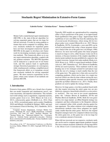
Stochastic Regret Minimization in Extensive-Form GamesGoofspiel, external sampling, 50 seedsMCCFRFTRL (η 10)OMD (η 10)Saddle-point gap1000.51.01.52.02.53.0Saddle-point gapBattleship, external sampling, 50 seedsMCCFRFTRL (η 100)OMD (η 10)1003.50.5Number of nodes touched ( 107 )1.52.02.5Search game (4 turns), external sampling, 50 seedsMCCFRFTRL (η 10)OMD (η 1)100Saddle-point gapLeduc13, external sampling, 50 seedsSaddle-point gap1.0Number of nodes touched ( 106 )MCCFRFTRL (η 100)OMD (η 1)10010 110 112345678Number of nodes touched ( 106 )0.20.40.60.81.0Number of nodes touched ( 106 )Figure 3. Performance of MCCFR, FTRL, and OMD when using the external sampling gradient estimator.Leduc13. Leduc13 uses a deck of 13 unique cards, with twocopies of each card. The game has 166,336 nodes and 6,007sequences per player.Goofspiel The variant of Goofspiel (Ross, 1971) that we usein our experiments is a two-player card game, employingthree identical decks of 4 cards each. This game has 54,421nodes and 21,329 sequences per player.Search is a security-inspired pursuit-evasion game. Thegame is played on a graph shown in Figure 5 in Ap
Stochastic Regret Minimization in Extensive-Form Games We denote by Xand Ythe set of all sequence-form strategies for Player 1 and Player 2, respectively.We denote by c the fixed sequence-form strategy of the chance player. For any leaf z2Z, the probability that the game ends in is the product of the probabilities of all the actions on the path