Transcription
Regret based Robust Solutions forUncertain Markov Decision ProcessesAsrar AhmedSingapore Management Universitymasrara@smu.edu.sgPradeep VarakanthamSingapore Management Universitypradeepv@smu.edu.sgYossiri AdulyasakMassachusetts Institute of Technologyyossiri@smart.mit.eduPatrick JailletMassachusetts Institute of Technologyjaillet@mit.eduAbstractIn this paper, we seek robust policies for uncertain Markov Decision Processes (MDPs). Mostrobust optimization approaches for these problems have focussed on the computation of maximinpolicies which maximize the value corresponding to the worst realization of the uncertainty. Recentwork has proposed minimax regret as a suitable alternative to the maximin objective for robust optimization. However, existing algorithms for handling minimax regret are restricted to models withuncertainty over rewards only. We provide algorithms that employ sampling to improve across multiple dimensions: (a) Handle uncertainties over both transition and reward models; (b) Dependenceof model uncertainties across state, action pairs and decision epochs; (c) Scalability and qualitybounds. Finally, to demonstrate the empirical effectiveness of our sampling approaches, we provide comparisons against benchmark algorithms on two domains from literature. We also provide aSample Average Approximation (SAA) analysis to compute a posteriori error bounds.IntroductionMotivated by the difficulty in exact specification of reward and transition models, researchers haveproposed the uncertain Markov Decision Process (MDP) model and robustness objectives in solvingthese models. Given the uncertainty over the reward and transition models, a robust solution cantypically provide some guarantees on the worst case performance. Most of the research in computing robust solutions has assumed a maximin objective, where one computes a policy that maximizesthe value corresponding to the worst case realization [8, 4, 3, 1, 7]. This line of work has developed scalable algorithms by exploiting independence of uncertainties across states and convexity ofuncertainty sets. Recently, techniques have been proposed to deal with dependence of uncertainties [15, 6].Regan et al. [11] and Xu et al. [16] have proposed minimax regret criterion [13] as a suitable alternative to maximin objective for uncertain MDPs. We also focus on this minimax notion of robustnessand also provide a new myopic variant of regret called Cumulative Expected Regret (CER) thatallows for development of scalable algorithms.Due to the complexity of computing optimal minimax regret policies [16] , existing algorithms [12]are restricted to handling uncertainty only in reward models and the uncertainties are independentacross states. Recent research has shown that sampling-based techniques [5, 9] are not only efficientbut also provide a priori (Chernoff-Hoeffiding bounds) and a posteriori [14] quality bounds forplanning under uncertainty.In this paper, we also employ sampling-based approaches to address restrictions of existing approaches for obtaining regret-based solutions for uncertain MDPs . More specifically, we make the1
following contributions: (a) An approximate Mixed Integer Linear Programming (MILP) formulation with error bounds for computing minimum regret solutions for uncertain MDPs, where theuncertainties across states are dependent. We further provide enhancements and error bounds toimprove applicability. (b) We introduce a new myopic concept of regret, referred to as CumulativeExpected Regret (CER) that is intuitive and that allows for development of scalable approaches.(c) Finally, we perform a Sample Average Approximation (SAA) analysis to provide experimentalbounds for our approaches on benchmark problems from literature.PreliminariesWe now formally define the two regret criterion that will be employed in this paper. In the definitionsbelow, we assume an underlying MDP, M hS, A, T, R, Hi where a policy is represented as: π t {π t , π t 1 , . . . , π H 1 }, the optimal policy as π and the optimal expected value as v 0 ( π ).The maximum reward in any state s is denoted as R (s) maxa R(s, a). Throughout the paper,we use α(s) to denote the starting state distribution in state s and γ to represent the discount factor.Definition 1 Regret for any policy π 0 is denoted by reg( π 0 ) and is defined as:Xreg( π 0 ) v 0 ( π ) v 0 ( π 0 ), where v 0 ( π 0 ) α(s) · v 0 (s, π 0 ),sttv (s, π ) XihXT (s, a, s0 ) · v t 1 (s0 , π t 1 )π (s, a) · R(s, a) γts0aExtending the definitions of simple and cumulative regret in stochastic multi-armed bandit problems [2], we now define a new variant of regret called Cumulative Expected Regret (CER).Definition 2 CER for policy π 0 is denoted by creg( π 0 ) and is defined as:Xcreg( π 0 ) α(s) · creg 0 (s, π 0 ), wheresttcreg (s, π ) XX π t (s, a) · R (s) R(s, a) γT (s, a, s0 ) · creg t 1 (s0 , π t 1 )as0(1)The following properties highlight the dependencies between regret and CER.hiH)Proposition 1 For a policy π 0 : 0 reg( π 0 ) creg( π 0 ) maxs R (s) mins R (s) · (1 γ1 γProof Sketch1 By rewriting Equation (1) as creg( π 0 ) v 0,# ( π 0 ) v 0 ( π 0 ), we provide the proof.Corollary 1 If s, s0 S : R (s) R (s0 ), then π 0 : creg( π 0 ) reg( π 0 ).Proof. Substituting maxs R (s) mins R (s) in the result of Proposition 1, we have creg( π 0 ) reg( π 0 ). Uncertain MDPA finite horizon uncertain MDP is defined as the tuple of hS, A, T, R, Hi. S denotes the set ofstates and A denotes the set of actions. T τ (T ) denotes a distribution over the set of transitionfunctions T , where Tkt (s, a, s0 ) denotes the probability of transitioning from state s S to state s0 S on taking action a A at time step t according to the kth element in T . Similarly, R ρ (R)denotes the distribution over the set of reward functions R, where Rtk (s, a, s0 ) is the reinforcementobtained on taking action a in state s and transitioning to state s0 at time t according to kth elementin R. Both T and R sets can have infinite elements. Finally, H is the time horizon.In the above representation, every element of T and R represent uncertainty over the entire horizonand hence this representation captures dependence in uncertainty distributions across states. We nowprovide a formal definition for the independence of uncertainty distributions that is equivalent to therectangularity property introduced in Iyengar et al. [4].1Detailed proof provided in supplement under Proposition 1.2
Definition 3 An uncertainty distribution τ over the set of transition functions, T is independentover state-action pairs at various decision epochs ifYtkt τ (T ) s S,a A,t H τ,tP r τ,t(Ts,a)s,a (Ts,a ), i.e. k, P r τ (T ) s,as,a,tt s,a,t Ts,a,tTs,akwhere T is the set of transition functions for s, a, t; τ,ts,a is the distribution overtthe set Ts,a and P r τ (T ) is the probability of the transition function T k given the distribution τ .We can provide a similar definition for the independence of uncertainty distributions over the reward functions. In the following definitions, we include transition, T and reward, R models assubscripts to indicate value (v), regret (reg) and CER (creg) functions corresponding to a specificMDP. Existing works on computation of maximin policies have the following objective:X0π maximin arg maxminα(s) · vT,R(s, π 0 )0T T ,R R πsOur goal is to compute policies that minimize the maximum regret or cumulative regret over possiblemodels of transitional and reward uncertainty.π reg arg minmax regT,R ( π 0 ); π creg arg minmax cregT,R ( π 0 )00T T ,R R π πT T ,R RRegret Minimizing SolutionWe will first consider the more general case of dependent uncertainty distributions. Our approachto obtaining regret minimizing solution relies on sampling the uncertainty distributions over thetransition and reward models. We formulate the regret minimization problem over the sample set asan optimization problem and then approximate it as a Mixed Integer Linear Program (MILP).We now describe the representation of a sample and the definition of optimal expected value fora sample, a key component in the computation of regret. Since there are dependencies amongstρ,tuncertainties, we can only sample from τ , ρ and not from τ,ts,a , s,a . Thus, a sample is:ξq { Tq0 , R0q , Tq1 , R1q , · · · TqH 1 , RqH 1 }where Tqt and Rtq refer to the transition and reward model respectively at time step t in sample q .Let π t represent the policy for each time step from t to H 1 and the set of samples be denotedby ξ. Intuitively, that corresponds to ξ number of discrete MDPs and our goal is to compute onepolicy that minimizes the regret over all the ξ MDPs, i.e.Xπ reg arg minmaxα(s) · [vξ q (s) vξ0q (s, π 0 )]0 πvξ qξq ξsvξ0q (s, π 0 )whereanddenote the optimal expected value and expected value for policy π 0 respectively of the sample ξq .Let, π 0 be any policy corresponding to the sample ξq , then the expected value is defined as follows:vξtq (s, π t ) Xπ t (s, a) · vξtq (s, a, π t ), where vξtq (s, a, π t ) Rtq (s, a) γXvξt 1(s0 , π t 1 ) · Tqt (s, a, s0 )qs0aThe optimization problem for computing the regret minimizing policy corresponding to sample setξ is then defined as follows:minreg( π 0 ) π0Xs.t. reg( π 0 ) vξ q α(s) · vξ0q (s, π 0 ) ξq(2)svξtq (s, π t ) Xtπ (s, a) · vξtq (s, a, π t ) s, ξq , t(3) s, a, ξq , t(4)avξtq (s, a, π t ) Rtq (s, a) γXvξt 1(s0 , π t 1 ) · Tqt (s, a, s0 )qs0The value function expression in Equation (3) is a product of two variables, π t (s, a) andvξtq (s, a, π t ), which hampers scalability significantly. We now linearize these nonlinear terms.3
Mixed Integer Linear ProgramThe optimal policy for minimizing maximum regret in the general case is randomized. However, toaccount for domains which only allow for deterministic policies, we provide linearization separatelyfor the two cases of deterministic and randomized policies.Deterministic Policy: In case of deterministic policies, we replace Equation (3) with the followingequivalent integer linear constraints:vξtq (s, π t ) vξtq (s, a, π t ) ; vξtq (s, π t ) π t (s, a) · Mvξtq (s, π t ) vξtq (s, a, π t ) (1 π t (s, a)) · M s, a, ξq , t(5)vξtq (s, a, π t ).tM is a large positive constant that is an upper bound onEquivalence to the productterms in Equation (3) can be verified by considering all values of π (s, a).Randomized Policy: When π 0 is a randomized policy, we have a product of two continuous variables. We provide a mixed integer linear approximation to address the product terms above. Let,vξt (s, a, π t ) π t (s, a)vξt (s, a, π t ) π t (s, a) t; Bξq (s, a, π t ) qAtξq (s, a, π t ) q22Equation (3) can then be rewritten as:Xvξtq (s, π t ) [Atξq (s, a, π t )2 Bξtq (s, a, π t )2 ](6)aAs discussed in the next subsection on “Pruning dominated actions”, we can compute upper andlower bounds for vξtq (s, a, π t ) and hence for Atξq (s, a, π t ) and Bξtq (s, a, π t ). We approximate thesquared terms by using piecewise linear components that provide an upper bound on the squaredterms. We employ a standard method from literature of dividing the variable range into multiplebreak points. More specifically, we divide the overall range of Atξq (s, a, π t ) (or Bξtq (s, a, π t )), say[br0 , brr ] into r intervals by using r 1 points namely hbr0 , br1 , . . . , brr i. We associate a linear vari22able, λtξq (s, a, w) with each break point w and then approximate Atξq (s, a, π t ) (and Bξtq (s, a, π t ) )as follows:XAtξq (s, a, π t ) λtξq (s, a, w) · brw , s, a, ξq , t(7)wAtξq (s, a, π t )2 Xλtξq (s, a, w) · (brw )2 , s, a, ξq , t(8) s, a, ξq , t(9)wXλtξq (s, a, w) 1,wtSOS2s,a,tξq ({λξq (s, a, w)}w r ), s, a, ξq , twhere SOS2 is a construct which is associated with a set of variables of which at most two variablescan be non-zero and if two variables are non-zero they must be adjacent. Since any number in therange lies between at most two adjacent points, we have the above constructs for the λtξq (s, a, w)variables. We implement the above adjacency constraints on λtξq (s, a, w) using the CPLEX SpecialOrdered Sets (SOS) type 22 .Proposition 2 Let [c,d] denote the range of values for Atξq (s, a, π t ) and assume we have r 1points that divide Atξq (s, a, π t )2 into r equal intervals of size error δ 4 .d2 c2rthen the approximationProof: Let the r 1 points be br0 , . . . , brr . By definition, we have (brw )2 (brw 1 )2 . Becauseof the convexity of x2 function, the maximum approximation error in any interval [brw 1 , brw ]occurs at its mid-point3 . Hence, approximation error δ is given by: 2(brw )2 (brw 1 )2brw brw 1 2 · brw 1 · (brw 1 brw ) δ 224423Using CPLEX SOS-2 considerably improves runtime compared to a binary variables formulation.Proposition and proof provided in supplement as footnote 34
Proposition 3 Let v̂ξtq (s, π t ) denote the approximation of vξtq (s, π t ). Thenvξtq (s, π t ) A · · (1 γ H 1 ) A · · (1 γ H 1 ) v̂ξtq (s, π t ) vξtq (s, π t ) 4 · (1 γ)4 · (1 γ)Proof Sketch4 : We use the approximation error provided in Proposition 2 and propagate it throughthe value function update. Corollary 2 The positive and negative errors in regret are bounded by A · ·(1 γ H 1 )4·(1 γ)Proof. From Equation (2) and Proposition 3, we have the proof. Since the break points are fixed before hand, we can find tighter bounds (refer to Proof of Proposition 2). Also, we can further improve on the performance (both run-time and solution quality) of theMILP by pruning out dominated actions and adopting clever sampling strategies as discussed in thenext subsections.Pruning dominated actionsWe now introduce a pruning approach5 to remove actions that will never be assigned a positiveprobability in a regret minimization strategy. For every state-action pair at each time step, we definea minimum and maximum value function as follows:(s, a)vξt,minqvξt,max(s, a)qnoTqt (s, a, s0 ) · vξt 1,min(s0 ) ; vξt,min(s) mina vξt,min(s, a)qqqnoP Rtq (s, a) γ s0 Tqt (s, a, s0 ) · vξt 1,max(s0 ) ; vξt,max(s) maxa vξt,max(s, a)qqq Rtq (s, a) γPs0An action a0 is pruned if there exists the same action a over all samples ξq , such thatvξt,min(s, a) vξt,max(s, a0 ) a, ξqqqThe above pruning step follows from the observation that an action whose best case payoff is lessthan the worst case payoff of another action a cannot be part of the regret optimal strategy, since wecould switch from a0 to a without increasing the regret value. It should be noted that an action thatis not optimal for any of the samples cannot be pruned.Greedy samplingThe scalability of the MILP formulation above is constrained by the number of samples Q. So,instead of generating only the fixed set of Q samples from the uncertainty distribution over models,we generate more than Q samples and then pick a set of size Q so that samples are “as far apart”as possible. The key intuition in selecting the samples is to consider distance among samples asbeing equivalent to entropy in the optimal policies for the MDPs in the samples. For each decisionepoch, t, each state s and action a, we define P rξs,a,t (πξ t (s, a) 1) to be the probability that a isthe optimal action in state s at time t. Similarly, we define P rξs,a,t (πξ t (s, a) 0): P P t t1 π(s,a)(s,a)πξqξqξq ξqP rξs,a,t (πξ t (s, a) 1) ; P rξs,a,t (πξ t (s, a) 0) QQLet the total entropy of sample set, ξ ( ξ Q) be represented as S(ξ), thenX X S(ξ) P rξs,a,t (πξ t (s, a) z) · ln P rξs,a,t (πξ t (s, a) z)t,s,a z {0,1}We use a greedy strategy to select the Q samples, i.e. we iteratively add samples that maximizeentropy of the sample set in that iteration.It is possible to provide bounds on the number of samples required for a given error using themethods suggested by Shapiro et al. [14]. However these bounds are conservative and as we showin the experimental results section, typically, we only require a small number of samples.45Detailed proof in supplement under Proposition 3Pseudo code provided in the supplement under ”Pruning dominated actions” section.5
CER Minimizing SolutionThe MILP based approach mentioned in the previous section can easily be adapted to minimize themaximum cumulative regret over all samples when uncertainties across states are dependent:min creg( π 0 ) π0s.t. creg( π 0 ) Xα(s) · cregξ0q (s, π t ), ξqscregξtq (s, π t ) Xπ t (s, a) · cregξtq (s, a, π t ), s, t, ξq(10) s, a, t, ξq(11)atcregξtq (s, a, π t ) R ,tq (s) Rq (s, a) γXTqt (s, a, s0 ) · cregξt 1(s0 , π t 1 ),qs0where the product term π t (s, a) · cregξtq (s, a, π t ) is approximated as described earlier.While we were unable to exploit the independence of uncertainty distributions across states withminimax regret, we are able to exploit the independence with minimax CER. In fact, a key advantageof the CER robustness concept in the context of independent uncertainties is that it has the optimalsubstructure over time steps and hence a Dynamic Programming(DP) algorithm can be used to solveit.In the case of independent uncertainties, samples at each time step can be drawn independently andwe now introduce a formal notation to account for samples drawn at each time step. Let ξ t denotethe set of samples at time step t, then ξ t H 1 ξ t . Further, we use ξ t to indicate cross productof samples from t to H 1, i.e. ξ t t e H 1 ξ e . Thus, ξ 0 ξ. To indicate the entire horizonsamples corresponding to a sample p from time step t, we have ξ pt ξpt ξ t 1 . ,t 1(s) Rt 1For notational compactness, we use Rt 1p (s, a). Because of indepenp (s, a) Rpt 1dence in uncertainties across time steps, for a sample set ξ p ξpt 1 ξ t , we have the following:Xπ t 1 ) maxmax cregξ t 1t 1 (s, t 1 pξt 1tξp ξpp maxt 1ξpXhiX tπ t 1 (s, a) Rt 1Tp (s, a, s0 ) · cregξ t t (s0 , π t )p (s, a) γs0aπt 1hiX t(s, a) Rt 1Tp (s, a, s0 ) · max cregξ t t (s0 , π t )p (s, a) γq t ξ tξqs0a(12)Proposition 4 At time step t 1, the CER corresponding to any policy π t 1 will have least regretif it includes the CER minimizing policy from t. Formally, if π ,t represents the CER minimizingpolicy from t and π t represents any arbitrary policy, then: t 1t 1 s : max creg t 1, π ,t max creg t 1, π t(13)t 1 s, πt 1 s, πξ pt 1 ξ t 1ξpif, s :ξ pt 1 ξ t 1max cregξ t t (s, π ,t )q ξqt ξ t ξpmax cregξ t t (s, π t )q ξqt ξ t(14)Proof Sketch6 We prove this by using Equations (14) and (12) in LHS of Equation (13). It is easy to show that minimizing CER also has an optimal substructure:XX minmaxα(s) · cregξ 00 (s, π 0 ) minα(s) · max cregξ 00 (s, π 0 )00 πξ p0s πpsξ p0(15)pIn Proposition 4 (extending the reasoning to t 1), we have already shown that maxξ 0 cregξ 00 (s, π 0 )pphas an optimal substructure. Thus, Equation (15) can also exploit the optimal substructure.M INIMIZE CER function below provides the pseudo code for a DP algorithm that exploits this structure. At each stage, t we calculate the creg for each state-action pair corresponding to each of the6Detailed proof in supplement under Proposition 4.6
samples at that stage, i.e. ξ t (lines 6-9). Once these are computed, we obtain the maximum creg andthe policy corresponding to it (line 10) using the G ET CER() function. In the next iteration, cregcomputed at t is then used in the computation of creg at t 1 using the same update step (lines 6-9).M INIMIZE CER()1: for all t H 1 do2:ξ t G EN S AMPLES(T, R)3: for all s S do4:creg H (s) 05: while t 0 do6:for all s S do7:for all ξqt ξ t , a A do8:cregξtqt (s, a) Rqt (s, a) P9:γ s0 Tqt (s, a, s0 ) · creg t 1 (s0 )10:π t , creg t (s) G ET CER (s, {cregξtqt (s, a)})11:t t 1return (creg 0 , π 0 )G ET CER (s, {cregξtqt (s, a)})min creg t (s)πX tcreg t (s) π (s, a) · cregξtqt (s, a), ξqtaXtπ (s, a) 1a0 π t (s, a) 1, aIt can be noted that M INIMIZE CER() makes only H · S calls to the LP in G ET CER() function,each of which has only A continuous variables and at most [1 maxt ξ t ] number of constraints.Thus, the overall complexity of MinimizeCER() is polynomial in the number of samples given fixedvalues of other attributes.Let creg ,H 1 (s, a) denote the optimal cumulative regret at time step H 1 for taking action a instate s and cregξ ,H 1 (s, a) denote the optimal cumulative regret over the sample set ξ. Let indicator(1 if creg ,H 1 (s, a) cregξ ,H 1 (s, a) λrandom variable, X be defined as follows: X 0 otherwiseBy using Chernoff and Hoeffding bounds on X, it is possible to provide bounds on deviation frommean and on the number of samples at H 1. This can then be propagated to H 2 and so on.However, these bounds can be very loose and they do not exploit the properties of creg functions.Bounds developed on spacings of order statistics can help exploit the properties of creg functions.We will leave this for future work.Experimental ResultsIn this section, we provide performance comparison of various algorithms introduced in previoussections over two domains. MILP-Regret refers to the randomized policy variant of the MILP approximation algorithm for solving uncertain MDPs with dependent uncertainties. Similar one forminimizing CER is referred to as MILP-CER. We refer to the dynamic programming algorithmfor minimizing CER in the independent uncertainty case as DP-CER and finally, we refer to themaximin value algorithm as “Maximin”. All the algorithms finished within 15 minutes on all theproblems. DP-CER was much faster than other algorithms and finished within a minute on thelargest problems.We provide the following results in this section:(1) Performance comparison of Greedy sampling and Random sampling strategies in the context ofMILP-Regret as we increase the number of samples.(2) SAA analysis of the results obtained using MILP-Regret.(3) Comparison of MILP-Regret and MILP-CER policies with respect to simulated regret.(4) Comparison of DP-CER and Maximin.The first three comparisons correspond to the dependent uncertainties case and the results are basedon a path planning problem that is motivated by disaster rescue and is a modification of the oneemployed in Bagnell et al. [1]. On top of normal transitional uncertainty, we have uncertainty overtransition and reward models due to random obstacles and random reward cells. Furthermore, theseuncertainties are dependent on each other due to patterns in terrains. Each sample of the variousuncertainties represents an individual map and can be modelled as an MDP. We experimented with7
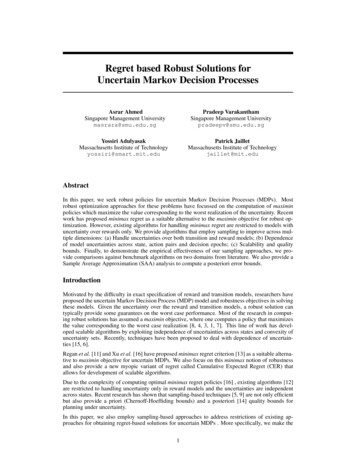
SAA AnalysisSampling Strategies (MILP-Regret)0.5Gap0.310.50.200.1 0.50 nceRandomGreedy0.6DifferenceDP-CER Analysis2.50.7DP-CER (0.3)Maximin (0.3)DP-CER (0.5)Maximin (0.5)DP-CER (0.7)Maximin .91Cost-to-revenue ratio(c)Figure 1: In (a),(b) we have 4 4 grid, H 5. In (c), the maximum inventory size (X) 50,H 20, ξ t 50. The normal distribution mean µ {0.3, 0.4, 0.5} · X and σ min{µ,X µ}3a grid world of size 4x4 while varying numbers of obstacles, reward cells, horizon and the numberof break points employed (3-6).In Figure 1a, we show the effect of using greedy sampling strategy on the MILP-Regret policy. OnX-axis, we represent the number of samples used for computation of policy (learning set). The testset from which the samples were selected consisted of 250 samples. We then obtained the policiesusing MILP-Regret corresponding to the sample sets (referred to as learning set) generated by usingthe two sampling strategies. On Y-axis, we show the percentage difference between simulated regretvalues on test and learning sample sets. We observe that for a fixed difference, the number of samplesrequired by greedy is significantly lower in comparison to random. Furthermore, the variance indifference is also much lower for greedy. A key result from this graph is that even with just 15samples, the difference with actual regret is less than 10%.Figure 1b shows that even the gap obtained using SAA analysis7 is near zero ( 0.1) with 15samples. We have shown the gap and variance on the gap over three different settings of uncertaintylabeled 1,2 and 3. Setting 3 has the highest uncertainty over the models and Setting 1 has the leastuncertainty. The variance over the gap was higher for higher uncertainty settings.While MILP-CER obtained a simulated regret value (over 250 samples) within the bound providedin Proposition 1, we were unable to find any correlation in the simulated regret values of MILPRegret and MILP-CER policies as the samples were increased. We have not yet ascertained a reasonfor there being no correlation in performance.In the last result shown in Figure 1c, we employ the well known single product finite horizon stochastic inventory control problem [10]. We compare DP-CER against the widely used benchmark algorithm on this domain, Maximin. The demand values at each decision epoch were taken from anormal distribution. We considered three different settings of mean and variance of the demand.As expected, the DP-CER approach provides much higher values than maximin and the differencebetween the two reduced as the cost to revenue ratio increased. We obtained similar results whenthe demands were taken from other distributions (uniform and bi-modal).ConclusionsWe have introduced scalable sampling-based mechanisms for optimizing regret and a new variant ofregret called CER in uncertain MDPs with dependent and independent uncertainties across states.We have provided a variety of theoretical results that indicate the connection between regret andCER, quality bounds on regret in case of MILP-Regret, optimal substructure in optimizing CER forindependent uncertainty case and run-time performance for MinimizeCER. In the future, we hope tobetter understand the correlation between regret and CER, while also understanding the propertiesof CER policies.Acknowledgement This research was supported in part by the National Research Foundation Singapore through the Singapore MIT Alliance for Research and Technologys Future Urban Mobilityresearch programme. The last author was also supported by ONR grant N00014-12-1-0999.7We have provided the method for performing SAA analysis in the supplement.8
References[1] J. Andrew Bagnell, Andrew Y. Ng, and Jeff G. Schneider. Solving uncertain markov decisionprocesses. Technical report, Carnegie Mellon University, 2001.[2] Sébastien Bubeck, Rémi Munos, and Gilles Stoltz. Pure exploration in multi-armed banditsproblems. In Proceedings of the 20th international conference on Algorithmic learning theory,Algorithmic Learning Theory, 2009.[3] Robert Givan, Sonia Leach, and Thomas Dean. Bounded-parameter markov decision processes. Artificial Intelligence, 122, 2000.[4] G. Iyengar. Robust dynamic programming. Mathematics of Operations Research, 30, 2004.[5] Michael Kearns, Yishay Mansour, and Andrew Y. Ng. A sparse sampling algorithm for nearoptimal planning in large markov decision processes. Machine Learning, 49, 2002.[6] Shie Mannor, Ofir Mebel, and Huan Xu. Lightning does not strike twice: Robust MDPs withcoupled uncertainty. In International Conference on Machine Learning (ICML), 2012.[7] Andrew Mastin and Patrick Jaillet. Loss bounds for uncertain transition probabilities in markovdecision processes. In IEEE Annual Conference on Decision and Control (CDC), 2012, 2012.[8] Arnab Nilim and Laurent El Ghaoui. Ghaoui, l.: Robust control of markov decision processeswith uncertain transition matrices. Operations Research, 2005.[9] Joelle Pineau, Geoffrey J. Gordon, and Sebastian Thrun. Point-based value iteration: Ananytime algorithm for POMDPs. In International Joint Conference on Artificial Intelligence,2003.[10] Martin Puterman. Markov Decision Processes: Discrete Stochastic Dynamic Programming.John Wiley and Sons, 1994.[11] Kevin Regan and Craig Boutilier. Regret-based reward elicitation for markov decision processes. In Uncertainty in Artificial Intelligence, 2009.[12] Kevin Regan and Craig Boutilier. Robust policy computation in reward-uncertain MDPs usingnondominated policies. In National Conference on Artificial Intelligence (AAAI), 2010.[13] Leonard Savage. The Foundations of Statistics. Wiley, 1954.[14] A. Shapiro. Monte carlo sampling methods. In Stochastic Programming, volume 10 of Handbooks in Operations Research and Management Science. Elsevier, 2003.[15] Wolfram Wiesemann, Daniel Kuhn, and Ber Rustem. Robust markov decision processes.Mathematics of Operations Research, 38(1), 2013.[16] Huan Xu and Shie Mannor. Parametric regret in uncertain markov decision processes. In IEEEConference on Decision and Control, CDC, 2009.9
Regret based Robust Solutions for Uncertain Markov Decision Processes Asrar Ahmed Singapore Management University masrara@smu.edu.sg Pradeep Varakantham