Transcription
A TRIDENT SCHOLARPROJECT REPORTNO. 433A Modeling and Data Analysis of Laser Beam Propagation in the Maritime DomainbyMidshipman 1/C Benjamin C. Etringer, USNUNITED STATES NAVAL ACADEMYANNAPOLIS, MARYLANDThis document has been approved for publicrelease and sale; its distribution is limited.USNA-1531-2
U.S.N.A. --- Trident Scholar project report; no. 433 (2015)A MODELING AND DATA ANALYSIS OF LASER BEAM PROPAGATIONIN THE MARITIME DOMAINbyMidshipman 1/C Benjamin C. EtringerUnited States Naval AcademyAnnapolis, MarylandCertification of Adviser ApprovalProfessor Reza Malek-MadaniMathematics Department(signature)(date)Acceptance for the Trident Scholar CommitteeProfessor Maria J. SchroederAssociate Director of Midshipman Research(signature)(date)USNA-1531-2
Form ApprovedOMB No. 0704-0188REPORT DOCUMENTATION PAGEPublic reporting burden for this collection of information is estimated to average 1 hour per response, including the time for reviewing instructions, searching existing data sources, gathering and maintaining thedata needed, and completing and reviewing this collection of information. Send comments regarding this burden estimate or any other aspect of this collection of information, including suggestions for reducingthis burden to Department of Defense, Washington Headquarters Services, Directorate for Information Operations and Reports (0704-0188), 1215 Jefferson Davis Highway, Suite 1204, Arlington, VA 222024302. Respondents should be aware that notwithstanding any other provision of law, no person shall be subject to any penalty for failing to comply with a collection of information if it does not display a currentlyvalid OMB control number. PLEASE DO NOT RETURN YOUR FORM TO THE ABOVE ADDRESS.1. REPORT DATE (DD-MM-YYYY)2. REPORT TYPE3. DATES COVERED (From - To)05-18-20154. TITLE AND SUBTITLE5a. CONTRACT NUMBERA Modeling and Data Analysis of Laser Beam Propagation in the Maritime Domain5b. GRANT NUMBER5c. PROGRAM ELEMENT NUMBER6. AUTHOR(S)5d. PROJECT NUMBEREtringer, Benjamin Charles5e. TASK NUMBER5f. WORK UNIT NUMBER7. PERFORMING ORGANIZATION NAME(S) AND ADDRESS(ES)8. PERFORMING ORGANIZATION REPORTNUMBER9. SPONSORING / MONITORING AGENCY NAME(S) AND ADDRESS(ES)10. SPONSOR/MONITOR’S ACRONYM(S)U.S. Naval AcademyAnnapolis, MD 2140211. SPONSOR/MONITOR’S REPORTNUMBER(S)Trident Scholar Report no. 433 (2015)12. DISTRIBUTION / AVAILABILITY STATEMENTThis document has been approved for public release; its distribution is UNLIMITED.13. SUPPLEMENTARY NOTES14. ABSTRACTIn this project we investigate the impact of the maritime environment on the propagation of laser beams. This study primarily uses datacollected at the Naval Academy with the goal of quantifying the correlation between the statistics of the environmental parameters and thestatistics of laser beam intensity at the target. The project has two parts to it: 1) we present a computational analysis of different probabilitydensity function approximation techniques; and 2) we introduce preliminary steps towards developing a stochastic model for the maritimelaser beam propagation. In the first part of this work we apply three mathematical methods to construct the probability density function ofthe data: i) the Kernel Density Estimator (KDE) method, ii) the Barakat Method using lower-order moments, and iii) the Bayesian MixtureModel. We compare and contrast the features of the three approximation techniques, first in the context of a synthetic data whose true pdf isknown, and next in the context of the laser data. In the second task, we analyze how a complex medium causes the photons of the laser lightto behave differently than if they were acting in freespace, by focusing on the stochastic behavior that our data exhibits. We develop astochastic paraxial wave equation in order to have a mathematical model capable of accepting statistical parameters from the atmosphere asinput to allow us to investigate the statistical properties of light intensity at a specified target.15. SUBJECT TERMSlaser propagation, data analysis, Bayesian statistics, probability density function16. SECURITY CLASSIFICATION OF:a. REPORTb. ABSTRACT17. LIMITATIONOF ABSTRACTc. THIS PAGE18. NUMBEROF PAGES5919a. NAME OF RESPONSIBLE PERSON19b. TELEPHONE NUMBER (include areacode)Standard Form 298 (Rev. 8-98)Prescribed by ANSI Std. Z39.18
1AbstractIn this project we investigate the impact of the maritime environment on the propagation of laserbeams. This study primarily uses data collected at the Naval Academy with the goal of quantifying the correlation between the statistics of the environmental parameters and the statistics oflaser beam intensity at the target. The project has two parts to it: 1) we present a computationalanalysis of different probability density function approximation techniques; and 2) we introducepreliminary steps towards developing a stochastic model for the maritime laser beam propagation.In the first part of this work we apply three mathematical methods to construct the probability density function of the data: i) the Kernel Density Estimator (KDE) method, ii) the Barakat Methodusing lower-order moments, and iii) the Bayesian Mixture Model. We compare and contrast thefeatures of the three approximation techniques, first in the context of a synthetic data whose truepdf is known, and next in the context of the laser data. In the second task, we analyze how a complex medium causes the photons of the laser light to behave differently than if they were acting infreespace, by focusing on the stochastic behavior that our data exhibits. We develop a stochasticparaxial wave equation in order to have a mathematical model capable of accepting statistical parameters from the atmosphere as input to allow us to investigate the statistical properties of lightintensity at a specified target.Keywords: laser propagation, data analysis, Bayesian statistics, probability density function.
2AcknowledgmentsI take this opportunity to express sincere gratitude to all the faculty members who have guided methroughout my time at the Academy. In particular, this project required a great deal of work andwould not have been possible without the support and patience from my adviser, Professor RezaMalek-Madani. Thanks is also given to Professor Maria Schroeder and the Trident Committee fortheir support. Finally, I am deeply grateful for the support from my family and friends.
3ContentsAbstract1Acknowledgments2List of Figures51Introduction and Motivation72Laser Beam Propagation in Free Space92.1 Exact Solution of PWE in half-space . . . . . . . . . . . . . . . . . . . . . . . . . 103Review of Histogram and PDF Concepts133.1 Histograms . . . . . . . . . . . . . . . . . . . . . . . . . . . . . . . . . . . . . . 133.2 Normal "Gaussian" Probability Density Function . . . . . . . . . . . . . . . . . . 164Laser Data Conveyed Through Histograms184.1 Analysis of Nighttime Data Using Histograms . . . . . . . . . . . . . . . . . . . 184.2 Daytime Laser Data Analysis Using Histograms . . . . . . . . . . . . . . . . . . 205Barakat Method for Computing PDFs Using Lower-Order Moments6Kernel Density Method for Computing PDFs276.1 Kernel Method Implemented on Synthetic Data . . . . . . . . . . . . . . . . . . . 287Gaussian Mixture Method8Description of Comparison Methods and Implementation of PDF Approximation Techniques on Synthetic Data328.1 Kolmogorov-Smirnov (K-S) Test . . . . . . . . . . . . . . . . . . . . . . . . . . . 328.2 Least Squares Test . . . . . . . . . . . . . . . . . . . . . . . . . . . . . . . . . . 338.3 Hellinger Distance . . . . . . . . . . . . . . . . . . . . . . . . . . . . . . . . . . 338.4 Application of K-S Test and Least Squares Test on Kernel Method with SyntheticData from Gaussian Distribution . . . . . . . . . . . . . . . . . . . . . . . . . . . 348.5 Hellinger Distance on Synthetic Data . . . . . . . . . . . . . . . . . . . . . . . . . 372230
49Implementation and Comparison of PDF Approximation Techniques on Laser Data 409.1 Nighttime Laser Data . . . . . . . . . . . . . . . . . . . . . . . . . . . . . . . . . 409.2 Daytime Laser Data . . . . . . . . . . . . . . . . . . . . . . . . . . . . . . . . . . 4310 Solution to Paraxial Wave Equation with Stochastic Refraction Coefficient11 Conclusion11.1 Barakat . . . . . . . . . .11.2 Kernel . . . . . . . . . . .11.3 Gaussian Mixture Method11.4 Summary . . . . . . . . .46.4848484849AppendixBarakat Function . . . . . . . . . .ECDF Computation Function . . . .Final PDF Comparison . . . . . . .Gaussian Mixture Method FunctionHellinger Distance . . . . . . . . .Kernel Method Function . . . . . .PDF to CDF Converting Function .5151525354565758.
5List of Figures1.1Time Series Plot of Laser Data. . . . . . . . . . . . . . . . . . . . . . . . . . .2.1Contours of the intensity, i.e., V12 V22 at a fixed distance (z 1200 meters) fromthe aperture. This figure is obtained with parameter values λ 633 nanometers,F0 500 meters, W0 0.03 meters. . . . . . . . . . . . . . . . . . . . . . . . . 123.13.23.33.43.53.63.7Example of a histogram. . . . . . . .Histogram of Ages with 10 Bins. . .Histogram of Ages with 2 Bins. . . .Histogram of Ages with 50 Bins. . .Gaussian PDF with μ 0 and σ 1.Comparison of Different Values for μ.Comparison of Different Values for σ.4.14.24.34.44.54.64.74.8Histogram of Black Data with 10 Bins. . . . .Histogram of Black Data with 100 Bins. . . . .Histogram of Black Data with 1,000 Bins. . . .Histogram of Black Data with 10,000 Bins. . .Histogram of Daytime Laser Data with 10 Bins.Histogram of Black Data with 100 Bins. . . . .Histogram of Daytime Data with 1,000 Bins. .Histogram of Daytime Data with 10,000 Bins.5.1Barakat Method Implemented on Synthetic Data. . . . . . . . . . . . . . . . . . . 266.16.2Pictorial Representation of the Kernel Method. . . . . . . . . . . . . . . . . . . . 28Kernel Method Implemented on Synthetic Data. . . . . . . . . . . . . . . . . . . 297.1Gaussian Mixture Method Implemented on Synthetic Data with 13 Clusters.8.18.28.38.48.58.68.7K-S Test Implemented on 50 Synthetic Data Points from Gaussian Distribution.Comparison of Kernel CDF, ECDF, and Gaussian CDF. . . . . . . . . . . . .Zoomed in Comparison of Kernel CDF, ECDF, and Gaussian CDF. . . . . . .Barakat CDF Implemented on Synthetic Data. . . . . . . . . . . . . . . . . .Zoomed in Comparison of Barakat CDF, ECDF, and Gaussian CDF. . . . . . .Table of Average Hellinger Distance after 50 Simulations. . . . . . . . . . . .Table of Full Results of Hellinger Distances after 50 Simulations. . . . . . . .8.13141515161717. . . .1819191920202121. . . 31.33343536373738
68.8Visual Comparison of the Three Approximation Techniques Implemented on Synthetic Data. . . . . . . . . . . . . . . . . . . . . . . . . . . . . . . . . . . . . . . 399.19.241Time Series Function of Laser Intensity During Nighttime 1. . . . . . . . . . . . .Visual Comparison of the Three Approximation Techniques Implemented on Nighttime Data 1. . . . . . . . . . . . . . . . . . . . . . . . . . . . . . . . . . . . . .9.3 Time Series Function of Laser Intensity During Nighttime 2. . . . . . . . . . . . .9.4 Visual Comparison of the Three Approximation Techniques Implemented on Nighttime Data 2. . . . . . . . . . . . . . . . . . . . . . . . . . . . . . . . . . . . . .9.5 Visual Representation for Convergence of Barakat Method for Nighttime LaserData. . . . . . . . . . . . . . . . . . . . . . . . . . . . . . . . . . . . . . . . . .9.6 Time Series Function of Laser Intensity During Daytime 1. . . . . . . . . . . . .9.7 Visual Comparison of the Three Approximation Techniques Implemented on Daytime Data 1. . . . . . . . . . . . . . . . . . . . . . . . . . . . . . . . . . . . . .9.8 Time Series Function of Laser Intensity During Daytime 2. . . . . . . . . . . . .9.9 Visual Comparison of the Three Approximation Techniques Implemented on Daytime Data 2. . . . . . . . . . . . . . . . . . . . . . . . . . . . . . . . . . . . . .9.10 Visual Representation for Convergence of Barakat Method for Daytime Laser Data.45414142424344444410.1 Simulated Time Series Laser Data. . . . . . . . . . . . . . . . . . . . . . . . . . 4710.2 PDF of Simulated Time Series Laser Data. . . . . . . . . . . . . . . . . . . . . . 47
7Chapter 1Introduction and MotivationThe intensity of laser light plays an integral role in many naval applications. From laser-basedweapon systems to determining distances with Laser Range Finders, the Navy has much to gainfrom increased knowledge in this field. Philip Nielsen, in Effects of Directed Energy Weapons, [8],emphasizes the uses for lasers in naval weaponry. Andrews and Phillips, Laser Beam PropagationThrough Random Media, [1], develop the mathematical framework associated with laser beams,and we intend to use these principles in an effort to further investigate the mathematical propertiesof laser beams in the maritime domain. Our goal by the end of the project is to better understandand quantify the properties of laser light by analyzing the intensities of laser light after the lighthas traveled through complex media. It is well-known that fluctuations in air temperature, as wellas the presence of aerosols and other scatterers, impacts the direction of propagation of a beam aswell as the amount of power it may deposit on a target (see Chapter 2 of [1]).This project primarily deals with the mathematical and computational analysis of data collectedfrom a Helium-Neon laser. The data we analyze has already been collected by a group supervisedby Prof. S. Avramov-Zamurovic of the Weapons and Systems Engineering Department. The datais of light intensity and is collected from a field experiment, in which we have set up a laser andsensor in stationary locations on Sherman Field, located on the premises of the Naval Academy.Figure 2 shows a typical stochastic behavior of the signals in the data and our goal is to understandthe extent of the contribution of the atmospheric conditions to the stochastic behavior of lightintensity in signals such as the one in Figure 2. To that end, we will use the recorded atmosphericparameters, including humidity, precipitation, temperature, wind, and cloud cover, with the goalof correlating the propagation properties with the effects of the turbulence in the medium. Mostof the laser beam data we have is from a target that is stationed 375 meters from the propagationsource (see [6] for a detailed description of the data collection). We will analyze the environmentaldiversity in data, ranging from the ambient light (day or night) to the aerosol conditions (land vs.water); we will compute the statistical parameters of the data in order to construct its probabilitydensity function, with the goal of identifying the signature of the atmospheric turbulence in ourdata.The sensor that detects photons of light is capable of recording intensities of the laser beam ata rate of 10000 Hz. That rate is equivalent to taking a data point every 150 microseconds. Datais collected for approximately three minutes, resulting in over a million data points to work withfor each data set. The data is stored electronically, and then converted into a vector that can beinterpreted by MATLAB. Currently over 100 such data sets are available on file for a variety of
8different atmospheric scenarios, equating to more than 100 million data points for the intensity oflaser light. See Figure 1.1 for an example of a time series plot of laser data. This graph shows theintensity of a recorded laser beam at a single pixel on a sensor located 375 meters from the source.The duration of the time series is 180 seconds, at a time interval of 150 μs.Figure 1.1: Time Series Plot of Laser Data.The structure of this thesis is as follows: In Chapter 2 we review the structure of a laser beamin free space. In Chapter 3 we review concepts of histograms and probability density functions,and we will create histograms for our laser data in Chapter 4. In Chapter 5, the method of Barakatwill be introduced. Chapter 6 is dedicated to the Kernel Density Method. Chapter 7 consists of thecomputation related to the Gaussian Mixture Methods. Chapter 8 provides a comparison and contrast of the three methods for computing a pdf using synthetic data. Chapter 9 implements thesetechniques on real data collected in the maritime domain. Chapter 10 provides an introductioninto future research by computing a solution to the paraxial wave equation that with a stochasticrefraction coefficient. Chapter 11 is the conclusion section.
9Chapter 2Laser Beam Propagation in Free SpaceLight propagation is governed by Maxwell’s equations. Let {E, B} be the electric and magneticfield pair that defines light. Then in a region with no charges or currents, Maxwell’s equations are1 E,c2 t · B 0. B t · E 0, B E (2.1)(2.2)Here c is the speed of light and is related to the medium’s permittivity 0 and permeability μ0 byc2 1. 0 μ0In what follows, where we closely follow the development in Chapter 4 of [1], we will show thateach component of E and B satisfies the wave equation. To see this first take the curl of the secondequation in (2.1) and use the identity ( E) ( · E) ΔE, and the first equation in2.2), · E 0, to get ΔE ( B) tNext, use the first equation in (2.1), B c12 E, to eliminate B and get a single equation for tE:1 2EΔE 2 2 .c tThe above equation is the well-known and standard wave equation.A similar development shows that B satisfies the same wave equation. Since the equations arelinear, we conclude that each component of either E or B satisfies the scalar wave equation1 2uΔu 2 2 .(2.3)c tNext we look for special solutions of the wave equation (2.3), namely, monochromatic solutionsof the formr x, y, z u(r, t) v(r)eiωt ,After substituting the above template into (2.3), we see that v satisfies Helmholtz’s equation2Δv k v 0,ω2k 2.c2(2.4)
10Finally, we look for beam-like soluions, i.e.,v(r) V (r)eikz .(2.5)Note that the function V in (2.5 is complex-valued,i.e, V V1 iV2 . We substitute the template(2.5) into the Helmholtz equation (2.4) and getΔ V 2 2V V 0, 2ik2 z z2 where Δ x2 y 2 .One of the main assumptions of laser beam propagation theory (again, see Chapter 4, [1]) is the2assumption that the term zV2 is much smaller than 2ik V , an is therefore ignored in the above zequation, resulting in the partial differential equationΔ V 2ik V 0. z(2.6)The above equation is called the Paraxial Wave Equation (PWE). We emphasize again that thisequation is complex-valued.2.1Exact Solution of PWE in half-spaceContinuing to follow the material in Chapter 4 of [1], we now present the exact solution of (2.6)when V is known at the aperture z 0. It turns out that if V (x, y, 0) is Gaussian, a term that wewill define precisely in the next section, then V (x, y, z) remain Gaussian for all z: Letr2ikr2V (x, y, 0) A exp( 2 ),W02F0(2.7)where W0 and F0 are called the spot-size radius and the phase radius of curvature of the beam atz 0, then (2.6) has the exact solutionAr2kr2V (x, y, z) 2exp( i(φ )),W (z)22F (z)Λ0 Θ20(2.8)where Λ0 , called the refraction parameter, and Θ0 , the diffraction parameter, areΛ0 1 z,F0Λ0 2zkW02(2.9)and W and F , which are the spot-size radius of the beam and its phase radius of curvature at anyz, are Λ0W (z) W0 Λ20 Θ20 , φ tan 1(2.10)Θ0F (z) F0(Θ20 Λ20 )(θ0 1)Θ20 Λ20 Θ0 )(2.11)
11Figure 2.6 shows a typical instance of the solution of PWE. In this figure the contours of intensity (irradiance) of a laser beam are plotted at a fixed distance z for the aperture – the intensity oflight is defined as V 2 . As expected, the beam has kept its gaussian shape far from the aperture.This feature, that a beam starting out as a gaussian, and remaining gaussian for all values of z isa special feature of beams propagating in vacuum or free space. In the problems that we take upin this paper, the laser beams that propagate in the maritime domain must interact with the atmosphere and consequently the gaussian nature of the beam is destroyed. One of the main goals ofthis paper is to attempt to quantify the impact of the atmosphere on a laser beam based on the datawe collect from various experiments. The next chapter introduces some of the mathematical toolswe need for this quantification.Figure 2.6 is obtained by executing the following program in MATLAB:lambda 633*10 -9; k 2*pi/lambda;F0 500;W0 0.03;Theta0 inline(’1-z/F0’,’z’, ’F0’);Lambda0 inline(’2*z/k/W0 2’,’z’,’k’,’W0’);z 0:1200;TH Theta0(z,F0); LA Lambda0(z,k,W0);W W0*sqrt(TH. 2 LA. 2);figure(1)plot(z,W)title(’Graph of W’)F F0*(TH. 2 LA. 2).*(TH-1)./(TH. 2 LA. 2-TH);figure(2)plot(z,F)title(’Graph of F’)[X,Y] meshgrid(-0.05:0.001:0.05,-0.05:0.001:0.05);z 1200;TH Theta0(z,F0); LA Lambda0(z,k,W0);W W0*sqrt(TH. 2 LA. 2);Irradiance 1./(TH. 2 LA. 2).*exp(-2*(X. 2 Y. 2)./W. 2);figure(3)[c, h] �Contours of Irradiance at z 1200’)
12Figure 2.1: Contours of the intensity, i.e., V12 V22 at a fixed distance (z 1200 meters) from theaperture. This figure is obtained with parameter values λ 633 nanometers, F0 500 meters,W0 0.03 meters.
13Chapter 3Review of Histogram and PDF Concepts3.1HistogramsWe begin by analyzing the data using histograms. Histograms, arguably the most elementarymethod of analyzing data points, display the frequency of occurrence of a random variable in aninterval or bin. See Figure 3.1 for an example of a histogram, in which we take a sample of 400points from a normal distribution with mean 0 and standard deviation 1. We create ten equallyspaced bins and place the points in the corresponding bins to create our histogram. The MATLABcode used to create the histogram in Figure 3.1 is stated below: data randn(400,1); hist(data,10) title(’Normally Distributed Random Numbers’)Figure 3.1: Example of a histogram.In addition to being easy to create, histograms are not computationally strenuous. For example,we will see with later methods that it is computationally impossible to use all the data points of adata set, while, with histograms, we can use all the data points. Future methods will require us tocreate functions for each data point and sum the functions together. The summation can be com-
14putationally difficult if the sample size of our data is significantly high. However, with histograms,the points are simply placed into pre-allocated bins, which is not computationally difficult. Byusing all the data points in our data set, we ensure that we are not ignoring any crucial data points.The bin size corresponds to the width of each bar in the histogram. Perhaps the easiest way tounderstand bins is with an example. Consider the ages of 100 random individuals who are walkinginto a Wal-Mart, given below—synthetic Wal-Mart data was generated from a uniform distributionof integers from 0-99.A bin size of 10 would allow us to focus on the variation of customers whose ages range withina ten year period. For example, the first bin takes into account all customers between the ages of 0and 9, the second bin those whose ages range between 10 and 19, and so forth. Figure 3.2 showsthe histogram of the data:Figure 3.2: Histogram of Ages with 10 Bins.It is easy to see from the histogram that we had 17 people in the age range of 0-9 years old, and6 people in the age range of 40-49 years old. If we change the number of bins to fewer than ten,we lose some of the details of the variability that the data carries. Figure 3.3 shows the histogramwhen we use only two bins:
15Figure 3.3: Histogram of Ages with 2 Bins.Similarly, if we have too many bins, we can lose meaningful information contained in the data.In Figure 3.4, for example, there are holes in the histogram that depict a 0% probability of an individual walking into Wal-Mart between the ages of 16 and 18. However, we know that the data waspulled from a uniform distribution. Therefore, there should be just as much chance as seeing anindividual walk into Wal-Mart between the ages of 16-18 and 18-20. Hence, we need to decreasethe bin size in order to plot a more accurate histogram for the synthetic, uniformly distributed,Wal-Mart data.Figure 3.4: Histogram of Ages with 50 Bins.What we should see from the Wal-Mart example is that we need a sufficiently large number ofbins with our histograms in order to create a histogram that is well represented by the data, but notmake the number so large that we lose the overall shape that the histogram should display. We willdo the same process with our Laser Data later in Chapter 3.
163.2Normal "Gaussian" Probability Density FunctionA probability density function (pdf) is a function used for determining the probability of a continuous random variable; particularly the probability that a certain data point will fall between twovalues (a and b). In order to determine the probability, we compute the area under the curve of thepdf, or the integral from a to b. That is, a probability density function f (x) is defined as, P (a x b) baf (x)dx.By definition, the area under any pdf must equal 1. Which means P (x)dx 1(3.1) The cumulative density function (cdf) is used when comparing different pdfs using the KolmogorovSmironov (K-S) Test or Least Squares Test (described in Chapter 7). The cdf, F (x) is defined as, xF (x) f (t)dt.(3.2) Note that limx F (x) 0 and limx F (x) 1.The Gaussian pdf is perhaps the most commonly used pdf in statistics and physical applications. The Gaussian pdf is sometimes colloquially referred to as the "bell curve" based on its shape.The Gaussian pdf has two arguments: the mean (μ) and standard deviation (σ), and is given by thefollowing equation:(x μ)21f (x) e 2σ2 .(3.3)σ 2πThe standard Gaussian pdf has μ 0 and σ 1. See Figure 3.5.Figure 3.5: Gaussian PDF with μ 0 and σ 1.
17Let us note that μ R and σ R . We should also note that a change in μ corresponds to ahorizontal shift, or translation, of the pdf. In addition, a change in σ corresponds to a horizontalstretch of the pdf. See Figures 3.6 and 3.7 as a reference:Figure 3.6: Comparison of Different Values for μ.Figure 3.7: Comparison of Different Values for σ.We will use the Gaussian pdf extensively throughout the remainder of the paper in various waysto compute approximate data-driven pdfs. Both the Kernel Method and Gaussian Mixture Methoduse the Gaussian pdf as a basis for the approximate pdf.
18Chapter 4Laser Data Conveyed Through HistogramsFor this paper we will rely on two data sets, one collected during the daytime and the other atnighttime. The first data set that we will consider will be nighttime data. The data was taken inthe middle of the night, when there was little to no light interfering with the laser beam. We willuse this as our control for other sets of data. The other data set we will use is daytime data, whichwas collected while the sun was actively impacting the laser beam. The data was collected froma stationary sensor, located 375 meters away from the laser aperture, that recorded scalar intensityvalues at a rate of 10 kHz for three minutes. The wavelength of the laser beam is 633 nm.4.1Analysis of Nighttime Data Using HistogramsWe will begin by looking at a histogram with only 10 bins. See Figure 4.1. We can see that thehistogram above does not reveal much information about the data set other than giving us the upperand lower bounds. Therefore, we will increase the number of bins by an order of magnitude. Theresulting histogram, shown in Figure 4.2, reveals more information about the data, but still doesnot depict the features that some of the histograms with smaller bin sizes are able to depict.Figure 4.1: Histogram of Black Data with 10 Bins.
19Figure 4.2: Histogram of Black Data with 100 Bins.Figure 4.2 depicts the overall skewed nature of the pdf, but with over a million points of data,we can increase the number of bins by another order of magnitude in order to improve the shapeof our histogram. The resulting histogram, as seen in Figure 4.3.Figure 4.3: Histogram of Black Data with 1,000 Bins.The bins are so narrow now, that we can no longer distinguish well the lines that separate bins.We should note that the current histogram exhibits significantly more features than the histogramwith 10 bins. For example, we can now see two local maximums in our histogram plot with 1,000bins that we could not see with only 10 bins. To ensure that no other local maximums occur in thehistogram plot of the data, we should look at another histogram with 10,000 bins. See Figure 4.4for histogram:Figure 4.4: Histogram of Black Data with 10,000 Bins.
20Note that there is not much of a difference between the histogram with 1,000 bins vs. the histogram with 10,000 bins. Therefore, we will use the histogram with 1,000 bins for our analysislater in the paper.The following is the MATLAB code used to create the above histograms (example for 100 bins): laser ConvertedData.Data.MeasuredData(1, 4).Data; hist(laser,100) title(’Histogram for Black Data with 100 Bins’)4.2Daytime Laser Data Analysis Using HistogramsThe Daytime Laser Data was taken during the daytime with the same laser and sensor. The distances are the same (375 meters). We will now do th
A Modeling and Data Analysis of Laser Beam Propagation in the Maritime Domain by Midshipman 1/C Benjamin C. Etringer, USN UNITED STATES NAVAL ACADEMY ANNAPOLIS, MARYLAND . Certification of Adviser Approval Professor Reza Malek-Madani Mathematics Department _ (signature) _ (date) Acceptance for the Trident Scholar Committee .