Transcription
ASSESSMENT OF FATIGUE DAMAGE OF MATERIALS AT VERY HIGH FREQUENCYH.CachãoMechanical Engineering Department, Instituto Superior Técnico,Av. Rovisco Pais, 1049-001 Lisboa, PortugalABSTRACTThe main goal of this paper is to present the evaluation of the mechanical resistance of three materials(Copper, Gray Cast Iron and Steel 42CrMo4) in domain of gigacycle fatigue and characterize their fracturesurfaces. Here is present a description of the design and construction of the ultrasonic fatigue testingmachine where the tests were carried out. This machine allows the control and monitoring of some variablesand, working at 20 kHz of frequency, enables reaching the VHCF regime in a small period of time.Some difficulties have occurred when trying to obtain points for S-N curves in the VHCF regime, because ofthe small stress range in this regime, and it was also difficult obtaining fatigue cracks initiation in the insideof specimen.KEYWORDS: Very High Cycle Fatigue (VHCF); Ultrasonic Fatigue; Fatigue Life Prediction; S-N Curvewould take more than one year to reach 10E9cycles [1].1. INTRODUCTIONIn mechanical design, the S-N diagrams are usedto dimension metallic components in order toresist a given number of load cycles. The dataused to create these diagrams is acquired in thelaboratory by performing cyclic tests until therupture. The classic fatigue test equipment hassome operational restrictions due to thetechnology used in the design of those machines.These limitations are mainly based on time spentin the cyclic tests. Due to this issue, the number oftesting cycles was generally limited to 10E6 to10E7, reaching a stress limit. This limit was named“endurance limit” which is a horizontal line definedbeyond 10E7 cycles in the S-N curve. This limitled to infinite fatigue lives if the cyclic loading isunder that limit. This was well accepted until theemergence of new productive technologies andmaterials increase the required fatigue life range,being necessary fatigue data beyond the specificcycles to design mechanical components.Nevertheless, it was observed fatigue failuresbeyond 10E6 cycles, which led to conclude thenecessity to improve the S-N diagrams andeliminate the endurance limit [1].The newest ultrasonic fatigue test machines canachieve the 10E9 cycles in few hours, turningthese tests practicable, in a feasible way. Theadvantages of the ultrasonic tests associated tothe improvements in piezoelectric devices,became the ultrasonic fatigue testing an attractivetechnique used around the world to establish S-Ncurves in VHCF.The application of ultrasonic fatigue testing startedin 1911, when Hopkinson developed a firstelectromagnetic resonance system. The frequencyreached by his fatigue testing machine was 116Hz. Other researchers, like Jenkin and Lehmann,continued his job, and about forty years later, in1950, Mason presented to scientific community, anultrasonic fatigue testing machine with 20 kHz asworking frequency. In the attempt to reach higherfrequencies, Girard presents in 1959 a testingmachine with 92 kHz as testing frequency but, thistesting frequency had some inconvenients, beingthe Mason’s 20 kHz machine used as the basis formost modern ultrasonic fatigue testing machines[1].The necessity to increase performances in termsof lifetime and security in mechanical componentsor structures is the motivation for intense research.Have a proper knowledge of the damage andrupture mechanisms in materials fatigue at VHCFdomain is extremely important nowadays.However, using conventional fatigue testingmachine to carry out VHCF tests can be very timeconsuming; for instance, making a fatigue test withhydraulic machine at 30 Hz as working frequencyThe objective of this work is to present theultrasonic fatigue testing machine developed inInstituto Superior Técnico (IST) by Freitas et al. [2]and evaluate the mechanical resistance of threematerials (Copper, Gray Cast Iron and Steel42CrMo4), making tests at VHCF regime andshowing the results by S-N diagrams. Theobtained fracture surfaces are also presented andcharacterized.1
object. The laser has a 1250 mm/s measurementrange and frequency responses up to 30 MHz.To measure the strain in the middle of specimen isused a 350 Ω 0.35% resistance strain gauge atquarter-bridge.2. FATIGUE TESTING MACHINEAs mentioned before, the ultrasonic fatigue testingmachine used was developed in IST by Freitas etal. [2]. This machine is based on the already usedby other researchers, namely by Bathias [3], andconsists of a data acquisition device (DAQ), aLabView routine, a signal generator and aresonance system comprising four elements(piezoelectric actuator, booster, horn andspecimen).Figure 1 shows a scheme of machineimplemented at IST laboratory.The piezoelectric actuator converts electricalsignals into mechanical vibrations and needs to beheaded by one signal generator. The piezoelectricactuator used is a 2.2 kW Branson transducer with20 kHz as working frequency and 20µm peak topeak of maximum displacement. The generatordelivers to the transducer an electric signal with asinusoidal shape and predetermined resonantfrequency. The signal generator selected, is aBranson DC222 with [19.5 – 20.5] KHz as workingfrequency range. The resonant frequency isdetermined by the signal generator through afrequency scan.All resonant elements are mechanically connectedby a screw connection; the piezoelectric actuator isconnected to the booster who in turn is connectedto the horn. The specimen is connected to the endof the horn. These four elements form theresonant system of the testing machine.The objectives of using one horn, is amplifying thedisplacements delivered by the booster and allowthe connectivity between the specimen test andthe resonant system. The horn and the specimentest was designed with a finite element routine andmachined in the workshop.Figure 1 – Ultrasonic fatigue testing machine scheme2.1. Machine Elements2.2. MonitoringThe NI USB-6216, is a bus-powered USB M Seriesmultifunction data acquisition device (DAQ)optimized for fast sampling rates: 16 analogueinputs, 400 kS/s sampling rate, two analogueoutputs, 32 digital I/O lines, four programmableinput ranges ( 0.2 to 10 V) per channel, digitaltriggering and two counter/timers. This deviceperforms the interface between elements ofmonitoring (pyrometer, laser and strain gauge) andLabView routine.The machine calibration is implemented with therelation between the power applied and thedisplacement at specimen test extremities. Due tothe several amplification levels in the resonantsystem the laser is a useful tool which permits toachieve accurate results in the axial stresspredictionandmonitoringthespecimenmechanical behaviour during the fatigue test. Thefatigue test monitoring is performed with aLabView routine, which receive signals from themonitoring system through the DAQ device. Thisroutine determines the testing frequency,establishes the power delivered to thepiezoelectric actuator to achieve the desired axialtension, indicate the specimen temperature historyand the number of cycles at rupture time. Whenthe fatigue test is finished a summary with themonitoring history is shown. The figures 2 and 3show the windows of setup and history acquisition,respectively, of the LabView routine. Besides themonitoring,LabViewroutineallowsthetemperature and amplitude control [4].The pyrometer is used to monitor on-line thetemperature of the specimen and send thatinformation to the Labview routine through theDAQ device, so as to be performed its control.This pyrometer have a [- 40ºC to 600ºC] asmeasure range, the accuracy is about 1% or 1ºCand have a 150 ms as response time.The laser measures the displacement in thespecimen bottom along the fatigue test. Thepolytec laser, with two acquisition channels, usesthe LDVs (Laser Doppler Vibrometers) technologyfor measuring velocities from a single point of the2
L1 1 1 arctan coth( L2 ) tanh( L2 ) kk Where k , and (3)are parameters defined by:k 2 fEd(4) R 1arctan 2 L2 R1 (5) Figure 2 – Primary setup window of LabView routine 2 k2(6)Being R1 , R2 , L1 and L2 , specimen dimensions,represented in figure 4, with L L1 L2 , and f ,Ed and , the resonance frequency, dynamicelastic modulus and density, respectively.From equation 1 is obtained: cos(kL1 ) cosh( L2 ) sinh( x), 0 x L2 A0sinh( L2 )cosh( x)U ( x) A cos k L x ,L2 x L 0Figure 3 – Acquisition window of LabView routine3. ANALYTICAL SPECIMEN DESIGNDeriving this equation is obtained the strain:Under longitudinal resonance, the specimenbehaviour must satisfy the differential equation (1),determined by the equilibrium of forces. 2u ( x, t ) A' ( x) u ( x, t ) 2u ( x, t ) c 2A( x) x t 2 x2 cosh( x) cosh( x) sinh( x) sinh( x) , A0 ( L1 , L2 )cosh 2 ( x) kA0 sin k L x , L2 x L(8)(1)By Hooke’s Law is obtained the stress: cosh( x) cosh( x) sinh( x) sinh( x) , E d A0 ( L1 , L2 )cosh 2 ( x) ( x) E kA sin k L x , d 0A' ( x) U ' ( x) U ( x) 0A( x) c 0 x L2 ( x) From this equation is obtained the displacementamplitude U (x) equation, given by:2U ' ' ( x) (7)0 x L2L2 x L(9)(2)Being ( L1 , L2 ) defined by:The geometry of the pretended specimen test ispresented in figure 4. ( L1, L2 ) cos(kL1 ) cosh( L2 )sinh( L2 )(10)4. MATERIALSThe study materials have the following properties:Figure 4 – Schematic presentation of specimen testHaving the central part of the specimen, ahyperbolic cosine profile, its design is given byresonance length (L1) equation:CopperCast IronSteelDynamicElasticModulus[Pa]Density3[kg/m 62089802882331100Table 1 – Materials properties3
7 – To collect the data.7. RESULTS AND DISCUSSION5. SPECIMENS AND HORNFrom equation 3 are designed the specimens ofthree materials:7.1 Laser vs Strain GaugeThe laser is the equipment chosen becauseguarantees the signal monitorization, during alltest, unlike strain gauge, that may break after afew cycles. Laser has some disadvantages andhere is made a comparison with strain gage, adevice which is more reliable in terms ofmeasurement.To compare them it is shown a graphic power vs.displacement for each material, and a graphic withtheir errors.Figure 5 – Copper specimenFigure 6 – Gray cast iron specimenFigure 9 – Copper displacement vs Power graphicFigure 7 – Steel specimenThe horn is designed with the help of finiteelements software:Figure 10 – Cast iron displacement vs Power graphicFigure 8 – Horn6. WORKING PROCEDUREFigure 11 – Steel displacement vs Power graphic1 – To design specimen.2 – To polish the base and the central zone ofthe specimen.3 – To connect the specimen at resonancesystem and perform the laser focus andpyrometer, as well as set desiredtemperature range for the test.4 – To perform setup test through software.5 – To start the test.6 – After fracture the test is stoppedautomatically.Figure 12 – Error vs Power graphic for three materials4
The linearity presented in figures 1, 2 and 3 bystrain gage shows its greater reliable. Looking tofigure 4, we see a less than 5% error for lasermeasuring up to 30 % power. After 30 % power,increases measurements uncertainty degree,making unreliable by laser, the measurementsabove 30 % power. This error is associated tolaser measurement limitations, because it onlymeasures speeds up to 1250 mm/s, what in usedoperating frequency, correspond to 10 um ofmaximum displacement. In order to increase thisrange of measurements was performed a simplealgorithm, which contains errors associated, inparticular to values greater than 30% potency.This error makes impracticable the displacementmeasurement in steel fatigue tests, since this is ahigh-strength material, requiring high stresses andtherefore high displacements.Figure 14 – Cast iron S-N curve7.2 S-N CurvesTo carry out the S-N curves, were tested severalsamples of each material, being some at fixedpower and others with amplitude control.The stress value applied in the center of specimen(σ(0)) is obtained by the application ofdisplacement amplitude value (A0), measured atspecimen bottom, in equation 11. (0) Ed A0cos(kL1 ) cosh( L2 ) sinh( L2 )Figure 15 – Steel S-N curve with points obtained inservo-hydraulic testing machine(11)For the test with constant amplitude (amplitudecontrol), the value of the displacement amplitude,with which is computed the stress, is the defined intest beginning. For the test with fixed power, thisvalue was the average of values measured at theend of the test when some stabilization is reached.In the case of steel, because of the difficultydisplacements measuring, the tests were allperformed at fixed power. The stress value in thiscase, is computed by the aid of linearity observedin power evolution in relation to strain gagedisplacement.Figure 16 – Steel Power vs Cycles Number graphicwith points obtained in ultrasonic testing machineFigure 17 – Steel S-N curve with all pointsThe fact of stress range for VHCF regime to begreatly reduced, along with setting difficult ofapplied stress values in ultrasonic fatigue tests, ledto a quantity, less than desired, of obtained pointsin that regime.The obtained points are in expected range, i.e.,the applied stresses in specimens are in the elasticregime, of the respective materials, and itsfracture occurs for stresses around 50 % ofultimate tensile strength.Figure 13 – Copper S-N curve5
7.3 Fracture Surfacesthe fact that iron is a very fragile material. Thepresented surfaces correspond at two specimenswith different lifetimes, which show that thesurface characteristics do not depend on theregime where the fracture occurs.Fractures in VHCF regime may occur due tointernal or external cracks [1]. In this paper hasbeen proposed to observe fracture surfacesobtained in ultrasonic fatigue tests, in order toobserve the crack occurrence site.8.
The NI USB-6216, is a bus-powered USB M Series multifunction data acquisition device (DAQ) optimized for fast sampling rates: 16 analogue inputs, 400 kS/s sampling rate, two analogue outputs, 32 digital I/O lines, four programmable input ranges ( 0.2 to 10 V) per channel, digital triggering and two counter/timers. This device